arima

Create univariate autoregressive integrated moving average (ARIMA) model

Description

The arima function returns an arima object specifying the functional form and storing the parameter values of an ARIMA(p,D,q) linear time series model for a univariate response process y_t.

arima enables you to create variations of the ARIMA model, including:

• An autoregressive (AR(p)), moving average (MA(q)), or ARMA(p,q) model.

• A model containing multiplicative seasonal components (SARIMA(p,D,q)⨉(p_s,D_s,q_s)_s).

• A model containing a linear regression component for exogenous covariates (ARIMAX).

• A composite conditional mean and conditional variance model. For example, you can create an ARMA conditional mean model containing a GARCH conditional variance model (garch).

The key components of an arima object are the polynomial degrees (for example, the AR polynomial degree p and the degree of integration D) because they completely specify the model structure. Given polynomial degrees, all other parameters, such as coefficients and innovation-distribution parameters, are unknown and estimable unless you specify their values.

To estimate a model containing unknown parameter values, pass the model and data to estimate. To work with an estimated or fully specified arima object, pass it to an object function.

Alternatively, you can:

• Create and work with arima model objects interactively by using Econometric Modeler.

• Model serial correlation in a disturbance series of a regression model by creating a regression model with ARIMA errors. For more details, see regARIMA and Alternative ARIMA Model Representations.

Creation

Syntax

Mdl = arima

Mdl = arima(p,D,q)

Mdl = arima(Name,Value)

Description

Mdl = arima creates an ARIMA(0,0,0) model containing only an unknown constant and a series of iid Gaussian innovations with mean 0 and an unknown variance.

Mdl = arima(p,D,q) creates an ARIMA(p,D,q) model containing nonseasonal AR polynomial lags from 1 through p, the degree D nonseasonal integration polynomial, and nonseasonal MA polynomial lags from 1 through q.

This shorthand syntax provides an easy way to create a model template in which you specify the degrees of the nonseasonal polynomials explicitly. The model template is suited for unrestricted parameter estimation. After you create a model, you can alter property values using dot notation.

Mdl = arima(Name,Value) sets properties and polynomial lags using name-value pair arguments. Enclose each name in quotes. For example, 'ARLags',[1 4],'AR',{0.5 –0.1} specifies the values –0.5 and 0.1 for the nonseasonal AR polynomial coefficients at lags 1 and 4, respectively.

This longhand syntax allows you to create more flexible models. arima infers all polynomial degrees from the properties that you set. Therefore, property values that correspond to polynomial degrees must be consistent with each other.

Input Arguments

The shorthand syntax provides an easy way for you to create nonseasonal ARIMA model templates that are suitable for unrestricted parameter estimation. For example, to create an ARMA(2,1) model containing unknown coefficients and innovations variance, enter:

Mdl = arima(2,0,1);

To impose equality constraints on parameter values during estimation, or include seasonal components, set the appropriate property values using dot notation.

p — Nonseasonal autoregressive polynomial degree

nonnegative integer

Nonseasonal autoregressive polynomial degree, specified as a nonnegative integer.

Data Types: double

D — Degree of nonseasonal integration

nonnegative integer

Degree of nonseasonal integration (the degree of the nonseasonal differencing polynomial), specified as a nonnegative integer. D sets the property D.

Data Types: double

q — Nonseasonal moving average polynomial degree

nonnegative integer

Nonseasonal moving average polynomial degree, specified as a nonnegative integer.

Data Types: double

Name-Value Arguments

Specify optional pairs of arguments as Name1=Value1,...,NameN=ValueN, where Name is the argument name and Value is the corresponding value. Name-value arguments must appear after other arguments, but the order of the pairs does not matter.

Before R2021a, use commas to separate each name and value, and enclose Name in quotes.

The longhand syntax enables you to create seasonal models or models in which some or all coefficients are known. During estimation, estimate imposes equality constraints on any known parameters.

Example: 'ARLags',[1 4],'AR',{0.5 –0.1} specifies the nonseasonal AR polynomial $$1-0.5L^1+0.1L^4$$.

ARLags — Lags associated with nonseasonal AR polynomial coefficients

1:numel(AR) (default) | numeric vector of unique positive integers

Lags associated with the nonseasonal AR polynomial coefficients, specified as the comma-separated pair consisting of 'ARLags' and a numeric vector of unique positive integers. The maximum lag is p.

AR{j} is the coefficient of lag ARLags(j), where AR is the value of the property AR.

Example: ARLags=4 specifies the nonseasonal AR polynomial$$1-{\varphi }_4{L}^4$$.

Example: ARLags=1:4 specifies the nonseasonal AR polynomial$$1-{\varphi }_1{L}^1-{\varphi }_2{L}^2-{\varphi }_3{L}^3-{\varphi }_4{L}^4$$.

Example: ARLags=[1 4] specifies the nonseasonal AR polynomial $$1-{\varphi }_1{L}^1-{\varphi }_4{L}^4.$$

Data Types: double

MALags — Lags associated with nonseasonal MA polynomial coefficients

1:numel(MA) (default) | numeric vector of unique positive integers

Lags associated with the nonseasonal MA polynomial coefficients, specified as the comma-separated pair consisting of 'MALags' and a numeric vector of unique positive integers. The maximum lag is q.

MA{j} is the coefficient of lag MALags(j), where MA is the value of the property MA.

Example: MALags=3 specifies the nonseasonal MA polynomial $$1+{\theta }_3{L}^3$$.

Example: MALags=1:3 specifies the nonseasonal MA polynomial $$1+{\theta }_1{L}^1+{\theta }_2{L}^2+{\theta }_3{L}^3.$$

Example: MALags=[1 3] specifies the nonseasonal MA polynomial $$1+{\theta }_1{L}^1+{\theta }_3{L}^3$$.

Data Types: double

SARLags — Lags associated with seasonal AR polynomial coefficients

1:numel(SAR) (default) | numeric vector of unique positive integers

Lags associated with the seasonal AR polynomial coefficients, specified as the comma-separated pair consisting of 'SARLags' and a numeric vector of unique positive integers. The maximum lag is p_s.

SAR{j} is the coefficient of lag SARLags(j), where SAR is the value of the property SAR.

Specify SARLags as the periodicity of the observed data, and not as multiples of the Seasonality property. This convention does not conform to standard Box and Jenkins [1] notation, but it is more flexible for incorporating multiplicative seasonality.

Example: 'SARLags',[4 8] specifies the seasonal AR polynomial $$1-{\Phi }_4{L}^4-{\Phi }_8{L}^8.$$

Data Types: double

SMALags — Lags associated with seasonal MA polynomial coefficients

1:numel(SMA) (default) | numeric vector of unique positive integers

Lags associated with the seasonal MA polynomial coefficients, specified as the comma-separated pair consisting of 'SMALags' and a numeric vector of unique positive integers. The maximum lag is q_s.

SMA{j} is the coefficient of lag SMALags(j), where SMA is the value of the property SMA.

Specify SMALags as the periodicity of the observed data, and not as multiples of the Seasonality property. This convention does not conform to standard Box and Jenkins [1] notation, but it is more flexible for incorporating multiplicative seasonality.

Example: 'SMALags',4 specifies the seasonal MA polynomial $$1+{\Theta }_4{L}^4.$$

Data Types: double

Note

Polynomial degrees are not estimable. If you do not specify a polynomial degree, or arima cannot infer it from other specifications, arima does not include the polynomial in the model.

Properties

You can set writable property values when you create the model object by using name-value argument syntax, or after you create the model object by using dot notation. For example, to create a fully specified ARMA(2,1) model, enter:

Mdl = arima('Constant',1,'AR',{0.3 -0.15},'MA',0.2);
Mdl.Variance = 1;

Note

• NaN-valued properties indicate estimable parameters. Numeric properties indicate equality constraints on parameters during model estimation. Coefficient vectors can contain both numeric and NaN-valued elements.

• You can specify polynomial coefficients as vectors in any orientation, but arima stores them as row vectors.

P — Compound AR polynomial degree

Read-only: nonnegative integer

This property is read-only.

Compound AR polynomial degree, specified as a nonnegative integer.

P does not necessarily conform to standard Box and Jenkins notation [1] because P captures the degrees of the nonseasonal and seasonal AR polynomials (properties AR and SAR, respectively), nonseasonal integration (property D), and seasonality (property Seasonality). Explicitly, P = p + D + p_s + s. P conforms to Box and Jenkins notation for models without integration or a seasonal AR component.

P specifies the number of lagged observations required to initialize the AR components of the model.

Data Types: double

Q — Compound MA polynomial degree

Read-only: nonnegative integer

This property is read-only.

Compound MA polynomial degree, specified as a nonnegative integer.

Q does not necessarily conform to standard Box and Jenkins notation [1] because Q captures the degrees of the nonseasonal and seasonal MA polynomials (properties MA and SMA, respectively). Explicitly, Q = q + q_s. Q conforms to Box and Jenkins notation for models without a seasonal MA component.

Q specifies the number of lagged innovations required to initialize the MA components of the model.

Data Types: double

Description — Model description

string scalar | character vector

Model description, specified as a string scalar or character vector. arima stores the value as a string scalar. The default value describes the parametric form of the model, for example "ARIMAX(1,1,1) Model (Gaussian Distribution)".

Example: "Model 1"

Data Types: string | char

Distribution — Conditional probability distribution of innovation process ε_t

"Gaussian" (default) | "t" | structure array

Conditional probability distribution of the innovation process ε_t, specified as a string or structure array. arima stores the value as a structure array.

Distribution	String	Structure Array
Gaussian	"Gaussian"	struct('Name',"Gaussian")
Student’s t	"t"	struct('Name',"t",'DoF',DoF)

The 'DoF' field specifies the t distribution degrees of freedom parameter.

• DoF > 2 or DoF = NaN.

• DoF is estimable.

• If you specify "t", DoF is NaN by default. You can change its value by using dot notation after you create the model. For example, Mdl.Distribution.DoF = 3.

• If you supply a structure array to specify the Student's t distribution, then you must specify both the 'Name' and the 'DoF' fields.

Example: Distribution=struct('Name',"t",'DoF',10)

Constant — Model constant

NaN (default) | numeric scalar

Model constant, specified as a numeric scalar.

Example: 1

Data Types: double

AR — Nonseasonal AR polynomial coefficients

cell vector

Nonseasonal AR polynomial coefficients, specified as a cell vector. Cells contain numeric scalars or NaN values. A fully specified nonseasonal AR polynomial must be stable.

Coefficient signs correspond to the model expressed in difference-equation notation. For example, for the nonseasonal AR polynomial $$\varphi \left(L\right)=1-0.5L+0.1L^2,$$ specify 'AR',{0.5 –0.1}.

If you do not set the 'ARLags' name-value pair argument, AR{j} is the coefficient of lag j, j = 1,…,p, where p = numel(AR).

Otherwise, p = max(ARLags) and the following conditions apply:

• The lengths of AR and ARLags must be equal.

• AR{j} is the coefficient of lag ARLags(j), for each j.

• arima stores AR as a length p cell vector. All cells that do not correspond to lags in ARLags contain 0.

The default value of AR depends on other specifications:

• If you use the shorthand syntax to specify p > 0, AR is a length p cell vector, where each cell contains a NaN value.

• If you specify ARLags, AR is a length p cell vector. AR{j} = NaN for each lag ARLags(j). All other cells contain 0.

• Otherwise, AR is an empty cell vector {}, meaning the model does not contain a nonseasonal AR polynomial.

The coefficients in AR correspond to coefficients in an underlying LagOp lag operator polynomial, and are subject to a near-zero tolerance exclusion test. If a coefficient is 1e–12 or below, arima excludes that coefficient and its corresponding lag in ARLags from the model.

Example: {0.8}

Example: {NaN –0.1}

Data Types: cell

SAR — Seasonal AR polynomial coefficients

cell vector

Seasonal AR polynomial coefficients, specified as a cell vector. Cells contain numeric scalars or NaN values. A fully specified seasonal AR polynomial must be stable.

Coefficient signs correspond to the model expressed in difference-equation notation. For example, for the seasonal AR polynomial $$\Phi \left(L\right)=1-0.5L^4+0.1L^8,$$ specify 'SAR',{0.5 –0.1}.

If you do not set the 'SARLags' name-value pair argument, SAR{j} is the coefficient of lag j, j = 1,…,p_s, where p_s = numel(SAR).

Otherwise, p_s = max(SARLags) and the following conditions apply:

• The lengths of SAR and SARLags must be equal.

• SAR{j} is the coefficient of lag SARLags(j), for each j.

• arima stores SAR as a length p_s cell vector. All cells that do not correspond to lags in SARLags contain 0.

The default value of SAR depends on the value SARLags:

• If you specify SARLags, SAR is a length p_s cell vector. SAR{j} = NaN for each lag SARLags(j). All other cells contain 0.

• Otherwise, SAR is an empty cell vector {}, meaning the model does not contain a seasonal AR polynomial.

The coefficients in SAR correspond to coefficients in an underlying LagOp lag operator polynomial, and are subject to a near-zero tolerance exclusion test. If a coefficient is 1e–12 or below, arima excludes that coefficient and its corresponding lag in SARLags from the model.

Example: {0.2 0.1}

Example: {NaN 0 0 NaN}

Data Types: cell

MA — Nonseasonal MA polynomial coefficients

cell vector

Nonseasonal MA polynomial coefficients, specified as a cell vector. Cells contain numeric scalars or NaN values. A fully specified nonseasonal MA polynomial must be invertible.

If you do not set the 'MALags' name-value pair argument, MA{j} is the coefficient of lag j, j = 1,…,q, where q = numel(MA).

Otherwise, q = max(MALags) and the following conditions apply:

• The lengths of MA and MALags must be equal.

• MA{j} is the coefficient of lag MALags(j), for each j.

• arima stores MA as a length q cell vector. All cells that do not correspond to lags in MALags contain 0.

The default value of MA depends on other specifications:

• If you use the shorthand syntax to specify q > 0, MA is a length q cell vector, where each cell contains a NaN value.

• If you specify MALags, MA is a length q cell vector. MA{j} = NaN for each lag MALags(j). All other cells contain 0.

• Otherwise, MA is an empty cell vector {}, meaning the model does not contain a nonseasonal MA polynomial.

The coefficients in SMA correspond to coefficients in an underlying LagOp lag operator polynomial, and are subject to a near-zero tolerance exclusion test. If a coefficient is 1e–12 or below, arima excludes that coefficient and its corresponding lag in SMALags from the model.

Example: 0.8

Example: {NaN –0.1}

Data Types: cell

SMA — Seasonal MA polynomial coefficients

cell vector

Seasonal MA polynomial coefficients, specified as a cell vector. Cells contain numeric scalars or NaN values. A fully specified seasonal MA polynomial must be invertible.

If you do not set the 'SMALags' name-value pair argument, SMA{j} is the coefficient of lag j, j = 1,…,q_s, where q_s = numel(SMA).

Otherwise, q_s = max(SMALags) and the following conditions apply:

• The lengths of SMA and SMALags must be equal.

• SMA{j} is the coefficient of lag SMALags(j), for each j.

• arima stores SMA as a length q_s cell vector. All cells that do not correspond to lags in SMALags contain 0.

The default value of SMA depends on other specifications:

• If you specify SMALags, SMA is a length q_s cell vector. SMA{j} = NaN for each lag SMALags(j). All other cells contain 0.

• Otherwise, SMA is an empty cell vector {}, meaning the model does not contain a seasonal MA polynomial.

The coefficients in SMA correspond to coefficients in an underlying LagOp lag operator polynomial, and are subject to a near-zero tolerance exclusion test. If a coefficient is 1e–12 or below, arima excludes that coefficient and its corresponding lag in SMALags from the model.

Example: {0.2 0.1}

Example: {NaN 0 0 NaN}

Data Types: cell

D — Degree of nonseasonal integration

0 (default) | nonnegative integer

Degree of nonseasonal integration, or the degree of the nonseasonal differencing polynomial, specified as a nonnegative integer.

Example: 1

Data Types: double

Seasonality — Degree of seasonal differencing polynomial

0 (default) | nonnegative integer

Degree of the seasonal differencing polynomial s, specified as a nonnegative integer.

Example: 12 specifies monthly periodicity.

Data Types: double

Beta — Regression component coefficients

empty row vector (default) | numeric vector

Regression component coefficients of the conditional mean, specified as a numeric vector.

If you plan to estimate all elements of Beta, you do not need to specify it. During estimation, estimate infers the size of Beta from the number of columns of the specified exogenous data X.

Example: [0.5 NaN 3]

Data Types: double

Variance — Model innovations variance

NaN (default) | positive scalar | supported conditional variance model object

Model innovations variance, specified as a positive scalar or a supported conditional variance model object (for example, garch). For all supported conditional variance models, see Conditional Variance Models.

A positive scalar or NaN specifies a homoscedastic model. A conditional variance model object specifies a composite conditional mean and variance model. estimate fits all unknown, estimable parameters in the composition.

Example: 1

Example: garch(1,0)

Data Types: double

SeriesName — Response series name

"Y" (default) | string scalar | character vector

Since R2023b

Response series name, specified as a string scalar or character vector. arima stores the value as a string scalar.

Example: "StockReturn"

Data Types: string | char

Object Functions

estimate	Fit univariate ARIMA or ARIMAX model to data
summarize	Display univariate ARIMA or ARIMAX model estimation results
infer	Infer univariate ARIMA or ARIMAX model residuals or conditional variances
filter	Filter disturbances using univariate ARIMA or ARIMAX model
impulse	Generate univariate ARIMA model impulse response function (IRF)
simulate	Monte Carlo simulation of univariate ARIMA or ARIMAX models
forecast	Forecast univariate ARIMA or ARIMAX model responses or conditional variances

Examples

Create Default Model

Create a default regression model with ARIMA errors by using regARIMA.

Mdl = regARIMA

Mdl = 
  regARIMA with properties:

     Description: "ARMA(0,0) Error Model (Gaussian Distribution)"
      SeriesName: "Y"
    Distribution: Name = "Gaussian"
       Intercept: NaN
            Beta: [1×0]
               P: 0
               Q: 0
              AR: {}
             SAR: {}
              MA: {}
             SMA: {}
        Variance: NaN

Mdl is an regARIMA object. Properties of the model appear at the command line.

The default model is

$$\begin{array}{l}{y}_t=c+u_t\\ u_t={\epsilon }_t,\end{array}$$

where $\mathit{c}$ is an unknown constant and ${\epsilon }_{\mathit{t}}$ is a series of iid Gaussian random variables with mean 0 and variance ${\sigma }^2$.

Mdl is a model template for estimation. You can modify property values by using dot notation or fit the model to data by using estimate, but you cannot pass Mdl to any other object function.

Create Default Model

Create a default ARIMA model by using arima.

Mdl = arima

Mdl = 
  arima with properties:

     Description: "ARIMA(0,0,0) Model (Gaussian Distribution)"
      SeriesName: "Y"
    Distribution: Name = "Gaussian"
               P: 0
               D: 0
               Q: 0
        Constant: NaN
              AR: {}
             SAR: {}
              MA: {}
             SMA: {}
     Seasonality: 0
            Beta: [1×0]
        Variance: NaN

Mdl is an arima object. Properties of the model appear at the command line.

The default model is

$$y_t=c+{\epsilon }_t$$,

where $\mathit{c}$ is an unknown constant and ${\epsilon }_{\mathit{t}}$ is a series of iid Gaussian random variables with mean 0 and variance ${\sigma }^2$.

Mdl is a model template for estimation. You can modify property values by using dot notation or fit the model to data by using estimate, but you cannot pass Mdl to any other object function.

Create Fully Specified Model

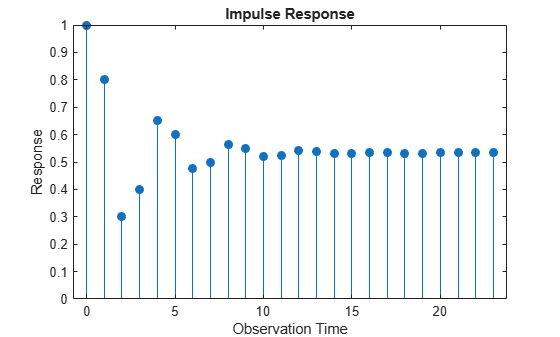
Create the ARIMA(2,1,1) model represented by this equation:

$$(1+0.5L^2)(1-L)y_t=3.1+(1-0.2L){\epsilon }_t,$$

where ${\epsilon }_{\mathit{t}}$ is a series of iid Gaussian random variables. Use the longhand syntax to specify parameter values in the equation written in difference-equation notation:

$$\Delta y_t=3.1-0.5\Delta y_{t-2}+{\epsilon }_t-0.2{\epsilon }_{t-1}.$$

Mdl = arima('ARLags',2,'AR',-0.5,'D',1,'MA',-0.2,...
    'Constant',3.1)

Mdl = 
  arima with properties:

     Description: "ARIMA(2,1,1) Model (Gaussian Distribution)"
      SeriesName: "Y"
    Distribution: Name = "Gaussian"
               P: 3
               D: 1
               Q: 1
        Constant: 3.1
              AR: {-0.5} at lag [2]
             SAR: {}
              MA: {-0.2} at lag [1]
             SMA: {}
     Seasonality: 0
            Beta: [1×0]
        Variance: NaN

Mdl is a fully specified arima object because all its parameters are known. You can pass Mdl to any arima object function except estimate. For example, plot the impulse response function of the model for 24 periods by using impulse.

impulse(Mdl,24)

Create Partially Specified Model

Create the AR(1) model represented by this equation:

$$y_t=1+\varphi y_{t-1}+{\epsilon }_t,$$

where ${\epsilon }_{\mathit{t}}$ is a series of iid Gaussian random variables with mean 0 and variance 0.5. Use the shorthand syntax to specify an AR(1) model template, then use dot notation to set the Constant and Variance properties.

Mdl = arima(1,0,0);
Mdl.Constant = 1;
Mdl.Variance = 0.5;
Mdl

Mdl = 
  arima with properties:

     Description: "ARIMA(1,0,0) Model (Gaussian Distribution)"
      SeriesName: "Y"
    Distribution: Name = "Gaussian"
               P: 1
               D: 0
               Q: 0
        Constant: 1
              AR: {NaN} at lag [1]
             SAR: {}
              MA: {}
             SMA: {}
     Seasonality: 0
            Beta: [1×0]
        Variance: 0.5

Mdl is a partially specified arima object. You can modify property values by using dot notation or fit the unknown coefficient $\varphi$ to data by using estimate, but you cannot pass Mdl to any other object function.

Create Nonseasonal ARIMA Model Template

Create the ARIMA(3,1,2) model represented by this equation:

$$(1-{\varphi }_{1}L-{\varphi }_2{L}^2-{\varphi }_3{L}^3)(1-L)y_t=(1+{\theta }_{1}L+{\theta }_2{L}^2){\epsilon }_t$$,

where ${\epsilon }_{\mathit{t}}$ is a series of iid Gaussian random variables with mean 0 and variance ${\sigma }^2$.

Because the model contains only nonseasonal polynomials, use the shorthand syntax.

Mdl = arima(3,1,2)

Mdl = 
  arima with properties:

     Description: "ARIMA(3,1,2) Model (Gaussian Distribution)"
      SeriesName: "Y"
    Distribution: Name = "Gaussian"
               P: 4
               D: 1
               Q: 2
        Constant: NaN
              AR: {NaN NaN NaN} at lags [1 2 3]
             SAR: {}
              MA: {NaN NaN} at lags [1 2]
             SMA: {}
     Seasonality: 0
            Beta: [1×0]
        Variance: NaN

The property P is equal to $$p$$ + $$D$$ = 4. NaN-valued elements indicate estimable parameters.

Specify Nonconsecutive Lags

To include additive seasonal lags, specify the lags matching the appropriate periodicity. For example, create the additive monthly MA(12) model represented in this equation:

$$y_t={\epsilon }_t+{\theta }_1{\epsilon }_{t-1}+{\theta }_{12}{\epsilon }_{t-12},$$

where ${\epsilon }_{\mathit{t}}$ is a series of iid Gaussian random variables with mean 0 and variance ${\sigma }^2$.

Mdl = arima('Constant',0,'MALags',[1 12])

Mdl = 
  arima with properties:

     Description: "ARIMA(0,0,12) Model (Gaussian Distribution)"
      SeriesName: "Y"
    Distribution: Name = "Gaussian"
               P: 0
               D: 0
               Q: 12
        Constant: 0
              AR: {}
             SAR: {}
              MA: {NaN NaN} at lags [1 12]
             SMA: {}
     Seasonality: 0
            Beta: [1×0]
        Variance: NaN

Create SARIMA Model Template

Create the SARIMA$\left(0,1,1\right)\times {\left(0,1,1\right)}_{12}$ model (multiplicative, monthly MA model template with one degree of seasonal and nonseasonal integration) represented by this equation:

$$(1-L)(1-L^{12})y_t=(1+{\theta }_{1}L)(1+{\theta }_{12}{L}^{12}){\epsilon }_t,$$

where ${\epsilon }_{\mathit{t}}$ is a series of iid Gaussian random variables with mean 0 and variance ${\sigma }^2$.

Mdl = arima('Constant',0,'D',1,'Seasonality',12,...
	'MALags',1,'SMALags',12)

Mdl = 
  arima with properties:

     Description: "ARIMA(0,1,1) Model Seasonally Integrated with Seasonal MA(12) (Gaussian Distribution)"
      SeriesName: "Y"
    Distribution: Name = "Gaussian"
               P: 13
               D: 1
               Q: 13
        Constant: 0
              AR: {}
             SAR: {}
              MA: {NaN} at lag [1]
             SMA: {NaN} at lag [12]
     Seasonality: 12
            Beta: [1×0]
        Variance: NaN

Modify Model Object

Create the AR(3) model represented by this equation:

$$y_t=0.05+0.6y_{t-1}+0.2y_{t-2}-0.1y_{t-3}+{\epsilon }_t,$$

where $${\epsilon }_t$$ is a series of iid Gaussian random variables with mean 0 and variance 0.01.

Mdl = arima('Constant',0.05,'AR',{0.6,0.2,-0.1},'Variance',0.01)

Mdl = 
  arima with properties:

     Description: "ARIMA(3,0,0) Model (Gaussian Distribution)"
      SeriesName: "Y"
    Distribution: Name = "Gaussian"
               P: 3
               D: 0
               Q: 0
        Constant: 0.05
              AR: {0.6 0.2 -0.1} at lags [1 2 3]
             SAR: {}
              MA: {}
             SMA: {}
     Seasonality: 0
            Beta: [1×0]
        Variance: 0.01

Add a nonseasonal MA term at lag 2 with coefficient 0.2. Then, display the MA property.

Mdl.MA = {0 0.2}

Mdl = 
  arima with properties:

     Description: "ARIMA(3,0,2) Model (Gaussian Distribution)"
      SeriesName: "Y"
    Distribution: Name = "Gaussian"
               P: 3
               D: 0
               Q: 2
        Constant: 0.05
              AR: {0.6 0.2 -0.1} at lags [1 2 3]
             SAR: {}
              MA: {0.2} at lag [2]
             SMA: {}
     Seasonality: 0
            Beta: [1×0]
        Variance: 0.01

Mdl.MA

ans=1×2 cell array
    {[0]}    {[0.2000]}

In the model display, lags indicates the lags to which the corresponding coefficients are associated. Although MATLAB® removes zero-valued coefficients from the display, the properties storing coefficients preserve them.

Change the model constant to 1.

Mdl.Constant = 1

Mdl = 
  arima with properties:

     Description: "ARIMA(3,0,2) Model (Gaussian Distribution)"
      SeriesName: "Y"
    Distribution: Name = "Gaussian"
               P: 3
               D: 0
               Q: 2
        Constant: 1
              AR: {0.6 0.2 -0.1} at lags [1 2 3]
             SAR: {}
              MA: {0.2} at lag [2]
             SMA: {}
     Seasonality: 0
            Beta: [1×0]
        Variance: 0.01

Specify t Distribution for Innovations

Create an AR(1) model template and specify iid $\mathit{t}$-distributed innovations with unknown degrees of freedom. Use the longhand syntax.

Mdl = arima('ARLags',1,'Distribution',"t")

Mdl = 
  arima with properties:

     Description: "ARIMA(1,0,0) Model (t Distribution)"
      SeriesName: "Y"
    Distribution: Name = "t", DoF = NaN
               P: 1
               D: 0
               Q: 0
        Constant: NaN
              AR: {NaN} at lag [1]
             SAR: {}
              MA: {}
             SMA: {}
     Seasonality: 0
            Beta: [1×0]
        Variance: NaN

The degrees of freedom DoF is NaN, which indicates that the degrees of freedom is estimable.

Create the fully specified AR(1) model represented by this equation:

$$y_t=0.6y_{t-1}+{\epsilon }_t,$$

where ${\epsilon }_{\mathit{t}}$ is an iid series of $\mathit{t}$-distributed random variables with 10 degrees of freedom. Use the longhand syntax.

innovdist = struct('Name',"t",'DoF',10);
Mdl = arima('Constant',0,'AR',{0.6},...
    'Distribution',innovdist)

Mdl = 
  arima with properties:

     Description: "ARIMA(1,0,0) Model (t Distribution)"
      SeriesName: "Y"
    Distribution: Name = "t", DoF = 10
               P: 1
               D: 0
               Q: 0
        Constant: 0
              AR: {0.6} at lag [1]
             SAR: {}
              MA: {}
             SMA: {}
     Seasonality: 0
            Beta: [1×0]
        Variance: NaN

Create Composite Conditional Mean and Variance Model Template

Create the ARMA(1,1) conditional mean model containing an ARCH(1) conditional variance model represented by these equations:

$$\begin{array}{l}{y}_t=c+\varphi y_{t-1}+{\epsilon }_t+\theta {\epsilon }_{t-1}.\\ {\epsilon }_t={\sigma }_t{z}_t.\\ {\sigma }_t^2=\kappa +\gamma {\sigma }_{t-1}^2.\\ z_t\sim N(0,1).\end{array}$$

Create the ARMA(1,1) conditional mean model template by using the shorthand syntax.

Mdl = arima(1,0,1)

Mdl = 
  arima with properties:

     Description: "ARIMA(1,0,1) Model (Gaussian Distribution)"
      SeriesName: "Y"
    Distribution: Name = "Gaussian"
               P: 1
               D: 0
               Q: 1
        Constant: NaN
              AR: {NaN} at lag [1]
             SAR: {}
              MA: {NaN} at lag [1]
             SMA: {}
     Seasonality: 0
            Beta: [1×0]
        Variance: NaN

The Variance property of Mdl is NaN, which means that the model variance is an unknown constant.

Create the ARCH(1) conditional variance model template by using the shorthand syntax of garch.

CondVarMdl = garch(0,1)

CondVarMdl = 
  garch with properties:

     Description: "GARCH(0,1) Conditional Variance Model (Gaussian Distribution)"
      SeriesName: "Y"
    Distribution: Name = "Gaussian"
               P: 0
               Q: 1
        Constant: NaN
           GARCH: {}
            ARCH: {NaN} at lag [1]
          Offset: 0

Create the composite conditional mean and variance model template by setting the Variance property of Mdl to CondVarMdl using dot notation.

Mdl.Variance = CondVarMdl

Mdl = 
  arima with properties:

     Description: "ARIMA(1,0,1) Model (Gaussian Distribution)"
      SeriesName: "Y"
    Distribution: Name = "Gaussian"
               P: 1
               D: 0
               Q: 1
        Constant: NaN
              AR: {NaN} at lag [1]
             SAR: {}
              MA: {NaN} at lag [1]
             SMA: {}
     Seasonality: 0
            Beta: [1×0]
        Variance: [GARCH(0,1) Model]

All NaN-valued properties of the conditional mean and variance models are estimable.

Estimate ARIMAX Model

Create an ARMAX(1,2) model for predicting changes in the US personal consumption expenditure based on changes in paid compensation of employees.

Load the US macroeconomic data set.

load Data_USEconModel

DataTimeTable is a MATLAB® timetable containing quarterly macroeconomic measurements from 1947:Q1 through 2009:Q1. PCEC is the personal consumption expenditure series, and COE is the paid compensation of employees series. Both variables are in levels. For more details on the data, enter Description at the command line.

The series are nonstationary. To avoid spurious regression, stabilize the variables by converting the levels to returns using price2ret. Compute the sample size.

pcecret = price2ret(DataTimeTable.PCEC);
coeret = price2ret(DataTimeTable.COE);
T = numel(pcecret);

Because conversion from levels to returns involves applying the first difference, the transformation reduces the total sample size by one observation.

Create an ARMA(1,2) model template using the shorthand syntax.

Mdl = arima(1,0,2);

The exogenous component enters the model during estimation. Therefore, you do not need to set the Beta property of Mdl to a NaN so that estimate fits the model to the data with the other parameters.

ARMA(1,2) process initialization requires Mdl.P = 1 observation. Therefore, the presample period is the first time point in the data (first row) and the estimation sample is the rest of the data. Specify variables identifying the presample and estimation periods.

idxpre = Mdl.P;
idxest = (Mdl.P + 1):T;

Fit the model to the data. Specify the presample by using the 'Y0' name-value pair argument, and specify the exogenous data by using the 'X' name-value pair argument.

EstMdl = estimate(Mdl,pcecret(idxest),'Y0',pcecret(idxpre),...
    'X',coeret(idxest));

 
    ARIMAX(1,0,2) Model (Gaussian Distribution):
 
                  Value      StandardError    TStatistic      PValue  
                _________    _____________    __________    __________

    Constant    0.0091866       0.001269         7.239      4.5203e-13
    AR{1}        -0.13506       0.081986       -1.6474        0.099478
    MA{1}       -0.090445       0.082052       -1.1023         0.27034
    MA{2}         0.29671       0.064589        4.5939      4.3505e-06
    Beta(1)        0.5831       0.048884        11.928      8.4535e-33
    Variance    5.305e-05     3.1387e-06        16.902      4.3581e-64

All estimates, except the lag 1 MA coefficient, are significant at 0.1 level.

Display EstMdl.

EstMdl

EstMdl = 
  arima with properties:

     Description: "ARIMAX(1,0,2) Model (Gaussian Distribution)"
      SeriesName: "Y"
    Distribution: Name = "Gaussian"
               P: 1
               D: 0
               Q: 2
        Constant: 0.00918662
              AR: {-0.135063} at lag [1]
             SAR: {}
              MA: {-0.0904453 0.296714} at lags [1 2]
             SMA: {}
     Seasonality: 0
            Beta: [0.583095]
        Variance: 5.30503e-05

Like Mdl, EstMdl is an arima model object representing an ARMA(1,2) process. Unlike Mdl, EstMdl is fully specified because it is fit to the data, and EstMdl contains an exogenous component, so it is an ARMAX(1,2) model.

Simulate ARIMA Model

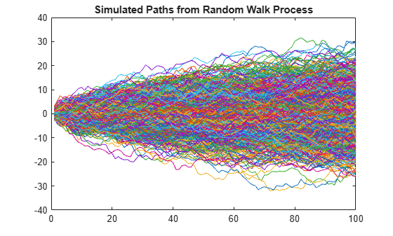
Create an arima model object for the random walk represented in this equation:

$$y_t=y_{t-1}+{\epsilon }_t,$$

where ${\epsilon }_{\mathit{t}}$ is a series of iid Gaussian random variables with mean 0 and variance 1.

Mdl = arima(0,1,0);
Mdl.Constant = 0;
Mdl.Variance = 1;
Mdl

Mdl = 
  arima with properties:

     Description: "ARIMA(0,1,0) Model (Gaussian Distribution)"
      SeriesName: "Y"
    Distribution: Name = "Gaussian"
               P: 1
               D: 1
               Q: 0
        Constant: 0
              AR: {}
             SAR: {}
              MA: {}
             SMA: {}
     Seasonality: 0
            Beta: [1×0]
        Variance: 1

Mdl is a fully specified arima model object.

Simulate and plot 1000 paths of length 100 from the random walk.

rng(1) % For reproducibility
Y = simulate(Mdl,100,'NumPaths',1000);
plot(Y)
title('Simulated Paths from Random Walk Process')

Forecast ARIMA Model

Forecast NASDAQ daily closing prices over a 500-day horizon.

Load the US equity indices data set.

load Data_EquityIdx

The data set contains daily NASDAQ closing prices from 1990 through 2001. For more details, enter Description at the command line.

Assume that an ARIMA(1,1,1) model is appropriate for describing the first 1500 NASDAQ closing prices. Create an ARIMA(1,1,1) model template.

Mdl = arima(1,1,1);

estimate requires a presample of size Mdl.P = 2.

Fit the model to the data. Specify the first two observations as a presample.

idxpre = 1:Mdl.P;
idxest = (Mdl.P + 1):1500;
EstMdl = estimate(Mdl,DataTable.NASDAQ(idxest),...
    'Y0',DataTable.NASDAQ(idxpre));

 
    ARIMA(1,1,1) Model (Gaussian Distribution):
 
                  Value      StandardError    TStatistic      PValue  
                _________    _____________    __________    __________

    Constant      0.43291       0.18607          2.3266       0.019989
    AR{1}       -0.076323      0.082045        -0.93026        0.35223
    MA{1}         0.31312      0.077284          4.0516     5.0876e-05
    Variance        27.86       0.63785          43.678              0

Forecast the closing values into a 500-day horizon by passing the estimated model to forecast. To initialize the model for forecasting, specify the last two observations in the estimation data as a presample.

yf0 = DataTable.NASDAQ(idxest(end - 1:end));
yf = forecast(EstMdl,500,yf0);

Plot the first 2000 observations and the forecasts.

dates = datetime(dates,'ConvertFrom',"datenum",...
    'Format',"yyyy-MM-dd");

figure
h1 = plot(dates(1:2000),DataTable.NASDAQ(1:2000));
hold on
h2 = plot(dates(1501:2000),yf,'r');
legend([h1 h2],"Observed","Forecasted",...
	     'Location',"NorthWest")
title("NASDAQ Composite Index: 1990-01-02 – 1997-11-25")
xlabel("Time (days)")
ylabel("Closing Price")
hold off

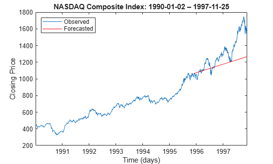
After the start of 1995, the model forecasts almost always underestimate the true closing prices.

More About

Lag Operator

The lag operator L is defined as $$L^i{y}_t=y_{t-i}.$$ Lag operators condense polynomial notation.

Linear Time Series Model

A linear time series model for response process y_t and random innovations ε_t is a stochastic process in which the current response is a linear function of previous responses, the current and previous innovations, and exogenous covariates x_t. In difference-equation notation, the general form of a linear time series model is:

$$y_t=c+x_t\beta +a_1{y}_{t-1}+\dots +a_w{y}_{t-w}+{\epsilon }_t+b_1{\epsilon }_{t-1}+\dots +b_v{\epsilon }_{t-v}.$$

Given w and v, all coefficients are estimable.

Expressed in lag operator notation, the general model form is:

$$a(L)y_t=c+x_t\beta +b(L){\epsilon }_t.$$

The lag operator polynomials in the model are often expressed as products of polynomials for nonseasonal and multiplicative seasonal effects and integration:

$$\varphi (L){(1-L)}^D\Phi (L){(1-L^s)}^{D_s}{y}_t=c+x_t\beta +\theta (L)\Theta (L){\epsilon }_t.$$

Model Component	Description	arima Property
$$\varphi (L)$$	$$\varphi (L)=1-\varphi L-{\varphi }_2{L}^2-\mathrm{...}-{\varphi }_p{L}^p,$$ a p-degree stable nonseasonal AR polynomial.	AR stores the coefficients; indices correspond to lag exponents.
D	Degree of nonseasonal integration	D
$$\Phi (L)$$	$$\Phi (L)=1-{\Phi }_{p_1}{L}^{p_1}-{\Phi }_{p_2}{L}^{p_2}-\mathrm{...}-{\Phi }_{p_s}{L}^{p_s},$$ a ps-degree stable, multiplicative seasonal AR polynomial.	SAR stores the coefficients; indices correspond to lag exponents.
s	Seasonality, or the degree of the seasonal differencing polynomial	Seasonality
Ds	Degree of seasonal integration	No corresponding property, but: If Seasonality > 0, Ds = 1. Otherwise, Ds = 0.
c	Model constant	Constant
β	Regression coefficient of exogenous covariates	Beta
$$\theta (L)$$	$$\theta (L)=1+\theta L+{\theta }_2{L}^2+\mathrm{...}+{\theta }_q{L}^q,$$ a q-degree invertible nonseasonal MA polynomial.	MA stores the coefficients; indices correspond to lag exponents.
$$\Theta (L)$$	$$\Theta (L)=1+{\Theta }_{q_1}{L}^{q_1}+{\Theta }_{q_2}{L}^{q_2}+\mathrm{...}+{\Theta }_{q_s}{L}^{q_s},$$ a qs-degree invertible, multiplicative seasonal MA polynomial.	SMA stores the coefficients; indices correspond to lag exponents.
εt	Series of random iid innovations	Distribution stores the distribution name and any parameters.

• The model property P is equal to p + D + p_s + s.

• The model property Q is equal to q + q_s.

Note

The degrees of the lag operators in the seasonal polynomials Φ(L) and Θ(L) do not conform to the degrees defined by Box and Jenkins [1]. In other words, Econometrics Toolbox™ does not treat p₁ = s, p₂ = 2s,...,p_s = r_ps and q₁ = s, q₂ = 2s,...,q_s = r_qs where r_p and r_q are positive integers. The software is flexible, letting you specify the lag operator degrees. See Create Multiplicative ARIMA Models.

Stationarity

A stochastic process y_t is stationary if its expected value, variance, and covariance between elements of the series are independent of time.

For example, the MA(q) model, with c = 0, is stationary for any $$q<\infty$$ because each of the following are free of t for all time points [1].

• $$E(y_t)=\theta (L)0=0.$$

• $$Var(y_t)={\sigma }^2{\displaystyle \sum _{i=1}^q{\theta }_i^2}.$$

• $$Cov(y_t,y_{t-s})=\{\begin{array}{l}{\sigma }^2({\theta }_s+{\theta }_1{\theta }_{s-1}+{\theta }_2{\theta }_{s-2}+\mathrm{...}+{\theta }_q{\theta }_{s-q})\text{ if }s\ge q\\ 0\text{ otherwise}.\end{array}$$

Unit Root

The time series $$\{y_t;t=1,\mathrm{...},T\}$$ is a unit root process if its expected value, variance, or covariance grows with time. Consequently, the time series is nonstationary.

References

[1] Box, George E. P., Gwilym M. Jenkins, and Gregory C. Reinsel. Time Series Analysis: Forecasting and Control. 3rd ed. Englewood Cliffs, NJ: Prentice Hall, 1994.

[2] Hamilton, James D. Time Series Analysis. Princeton, NJ: Princeton University Press, 1994.

Version History

Introduced in R2012a

R2023b: Name an ARIMA model response series

Name the response series of an ARIMA model by setting the SeriesName property to a string scalar. When you supply input response data to model object functions in a table or timetable, the functions choose the variable with name SeriesName as the response variable by default.

R2018a: Describe an ARIMA model

Describe an ARIMA model by setting the Description property to a string scalar.

R2018a: Use indices that are consistent with MATLAB cell array indexing

The indices of cell arrays of lag operator polynomial coefficients follow MATLAB^® cell array indexing rules. Affected model properties are AR, MA, SAR, and SMA.

• You cannot access any lag-zero coefficients by using an index of 0. For example, Mdl.AR{0} issues an error.

  Remove any instances of such zero indices from your code. The value of all lag-zero coefficients is 1, except for the lag operator polynomial corresponding to the ARCH property, which has the value 0.

• You cannot index beyond the maximal lag in the polynomial. For example, if Mdl.P is 4, then Mdl.AR{p} issues an error when p is greater than 4. For details on the maximal lags of the lag operator polynomials, see the corresponding property descriptions.

  Remove any instances of such indices beyond the maximal lag from your code. All coefficients beyond the maximal lag are 0.

R2018a: Models store innovation distribution name as a string scalar

The Name field of the Distribution property of arima model objects stores the innovation distribution name as a string scalar, for example, "Gaussian" for Gaussian innovations. Before R2018a, MATLAB stored the innovation distribution name as a character vector, for example 'Gaussian' for Gaussian innovations. Although most text-data operations accept character vectors and string scalars for text-data input, the two data types have some differences. For details, see Text in String and Character Arrays.