Voronoi Diagrams
The Voronoi diagram of a discrete set of points X decomposes
the space around each point X(i)
into a region of influence R{i}.
This decomposition has the property that an arbitrary point P within
the region R{i} is closer to
point i than any other point. The region of influence
is called a Voronoi region and the collection of all the Voronoi regions
is the Voronoi diagram.
The Voronoi diagram is an N-D geometric construct, but most practical applications are in 2-D and 3-D space. The properties of the Voronoi diagram are best understood using an example.
Plot 2-D Voronoi Diagram and Delaunay Triangulation
This example shows the Voronoi diagram and the Delaunay triangulation on the same 2-D plot.
Use the 2-D voronoi function to plot the Voronoi diagram for a set of points.
figure()
X = [-1.5 3.2; 1.8 3.3; -3.7 1.5; -1.5 1.3; ...
      0.8 1.2; 3.3 1.5; -4.0 -1.0;-2.3 -0.7; ...
      0 -0.5; 2.0 -1.5; 3.7 -0.8; -3.5 -2.9; ...
     -0.9 -3.9; 2.0 -3.5; 3.5 -2.25];

voronoi(X(:,1),X(:,2))

% Assign labels to the points.
nump = size(X,1);
plabels = arrayfun(@(n) {sprintf('X%d', n)}, (1:nump)');
hold on
Hpl = text(X(:,1), X(:,2), plabels, 'FontWeight', ...
      'bold', 'HorizontalAlignment','center', ...
      'BackgroundColor', 'none');

% Add a query point, P, at (0, -1.5).
P = [0 -1];
plot(P(1),P(2), '*r');
text(P(1), P(2), 'P', 'FontWeight', 'bold', ...
     'HorizontalAlignment','center', ...
     'BackgroundColor', 'none');
hold off
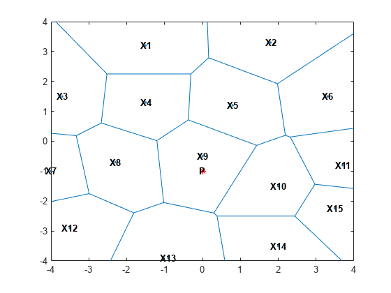
Observe that P is closer to X9 than to any other point in X, which is true for any point P within the region that bounds X9.
The Voronoi diagram of a set of points X is closely related to the Delaunay triangulation of X. To see this relationship, construct a Delaunay triangulation of the point set X and superimpose the triangulation plot on the Voronoi diagram.
dt = delaunayTriangulation(X);
hold on
triplot(dt,'-r');
hold off
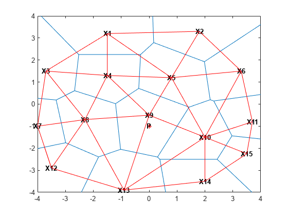
From the plot you can see that the Voronoi region associated with the point X9 is defined by the perpendicular bisectors of the Delaunay edges attached to X9. Also, the vertices of the Voronoi edges are located at the circumcenters of the Delaunay triangles. You can illustrate these associations by plotting the circumcenter of triangle {|X9|,|X4|,|X8|}.
To find the index of this triangle, query the triangulation. The triangle contains the location (-1, 0).
tidx = pointLocation(dt,-1,0);
Now, find the circumcenter of this triangle and plot it in green.
cc = circumcenter(dt,tidx);
hold on
plot(cc(1),cc(2),'*g');
hold off
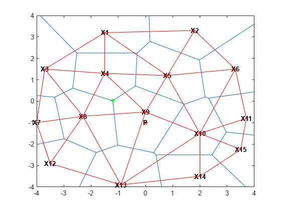
The Delaunay triangulation and Voronoi diagram are geometric duals of each other. You can compute the Voronoi diagram from the Delaunay triangulation and vice versa.
Observe that the Voronoi regions associated with points on the convex hull are unbounded (for example, the Voronoi region associated with X13). The edges in this region "end" at infinity. The Voronoi edges that bisect Delaunay edges (X13, X12) and (X13, X14) extend to infinity. While the Voronoi diagram provides a nearest-neighbor decomposition of the space around each point in the set, it does not directly support nearest-neighbor queries. However, the geometric constructions used to compute the Voronoi diagram are also used to perform nearest-neighbor searches.
Computing the Voronoi Diagram
This example shows how to compute a 2–D and 3–D Voronoi diagram.
MATLAB® provides functions to plot the Voronoi diagram in 2-D and to compute the topology of the Voronoi diagram in N-D. In practice, Voronoi computation is not practical in dimensions beyond 6-D for moderate to large data sets, due to the exponential growth in required memory.
The voronoi plot function plots the Voronoi
diagram for a set of points in 2-D space. In MATLAB there are
two ways to compute the topology of the Voronoi diagram of a point
set:
Using the function
voronoinUsing the
delaunayTriangulationmethod,voronoiDiagram.
The voronoin function
supports the computation of the Voronoi topology for discrete points
in N-D (N ≥ 2). The voronoiDiagram method
supports computation of the Voronoi topology for discrete points 2-D
or 3-D.
The voronoiDiagram method
is recommended for 2-D or 3-D topology computations as it is more
robust and gives better performance for large data sets. This method
supports incremental insertion and removal of points and complementary
queries, such as nearest-neighbor point search.
The voronoin function
and the voronoiDiagram method
represent the topology of the Voronoi diagram using a matrix format.
See Triangulation Matrix Format for
further details on this data structure.
Given a set of points, X, obtain the topology of the Voronoi diagram as follows:
Using the
voronoinfunction
[V,R] = voronoin(X)
Using the
voronoiDiagrammethod
dt = delaunayTriangulation(X);
[V,R] = voronoiDiagram(dt)
V is a matrix representing the coordinates of the Voronoi vertices (the vertices are the end points of the Voronoi edges). By convention the first vertex in V is the infinite vertex. R is a vector cell array length size(X,1), representing the Voronoi region associated with each point. Hence, the Voronoi region associated with the point X(i) is R{i}.
Define and plot the voronoi diagram for a set of points
X = [-1.5 3.2; 1.8 3.3; -3.7 1.5; -1.5 1.3; 0.8 1.2; ...
      3.3 1.5; -4.0 -1.0; -2.3 -0.7; 0 -0.5; 2.0 -1.5; ...
      3.7 -0.8; -3.5 -2.9; -0.9 -3.9; 2.0 -3.5; 3.5 -2.25];
[VX,VY] = voronoi(X(:,1),X(:,2));
h = plot(VX,VY,'-b',X(:,1),X(:,2),'.r');
xlim([-4,4])
ylim([-4,4])

% Assign labels to the points X.
nump = size(X,1);
plabels = arrayfun(@(n) {sprintf('X%d', n)}, (1:nump)');
hold on
Hpl = text(X(:,1), X(:,2)+0.2, plabels, 'color', 'r', ...
      'FontWeight', 'bold', 'HorizontalAlignment',...
      'center', 'BackgroundColor', 'none');

% Compute the Voronoi diagram.
dt = delaunayTriangulation(X);
[V,R] = voronoiDiagram(dt);


% Assign labels to the Voronoi vertices V.
% By convention the first vertex is at infinity.
numv = size(V,1);
vlabels = arrayfun(@(n) {sprintf('V%d', n)}, (2:numv)');
hold on
Hpl = text(V(2:end,1), V(2:end,2)+.2, vlabels, ...
      'FontWeight', 'bold', 'HorizontalAlignment',...
      'center', 'BackgroundColor', 'none');
hold off
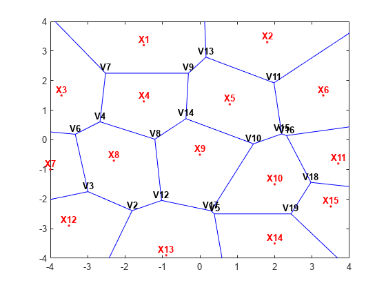
R{9} gives the indices of the Voronoi vertices associated with the point site X9.
R{9}ans = 1×5
8 12 17 10 14
The indices of the Voronoi vertices are the indices with respect to the V array.
Similarly, R{4} gives the indices of the Voronoi vertices associated with the point site X4.
R{4}ans = 1×5
4 8 14 9 7
In 3-D a Voronoi region is a convex polyhedron, the syntax for creating the Voronoi diagram is similar. However the geometry of the Voronoi region is more complex. The following example illustrates the creation of a 3-D Voronoi diagram and the plotting of a single region.
Create a sample of 25 points in 3-D space and compute the topology of the Voronoi diagram for this point set.
rng('default')
X = -3 + 6.*rand([25 3]);
dt = delaunayTriangulation(X);
Compute the topology of the Voronoi diagram.
[V,R] = voronoiDiagram(dt);
Find the point closest to the origin and plot the Voronoi region associated with this point.
tid = nearestNeighbor(dt,0,0,0);
XR10 = V(R{tid},:);
K = convhull(XR10);
defaultFaceColor  = [0.6875 0.8750 0.8984];
trisurf(K, XR10(:,1) ,XR10(:,2) ,XR10(:,3) , ...
        'FaceColor', defaultFaceColor, 'FaceAlpha',0.8)
title('3-D Voronoi Region')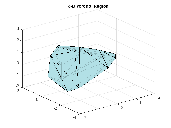
Related Topics
Select a Web Site
Choose a web site to get translated content where available and see local events and offers. Based on your location, we recommend that you select: United States.
You can also select a web site from the following list
Americas
- América Latina (Español)
- Canada (English)
- United States (English)
Europe
- Belgium (English)
- Denmark (English)
- Deutschland (Deutsch)
- España (Español)
- Finland (English)
- France (Français)
- Ireland (English)
- Italia (Italiano)
- Luxembourg (English)
- Netherlands (English)
- Norway (English)
- Österreich (Deutsch)
- Portugal (English)
- Sweden (English)
- Switzerland
- United Kingdom (English)
Asia Pacific
- Australia (English)
- India (English)
- New Zealand (English)
- 中国
- 日本Japanese (日本語)
- 한국Korean (한국어)