pdeeig
(Not recommended) Solve eigenvalue PDE problem
pdeeig
is not recommended. Use solvepdeeig
instead.
Description
[
produces the solution to the FEM formulation of the scalar PDE eigenvalue
problemv
,l
] =
pdeeig(model
,c
,a
,d
,r
)
or the system PDE eigenvalue problem
with geometry, boundary conditions, and mesh specified in
model
, a PDEModel
object.
The eigenvalue PDE problem is a homogeneous problem, i.e., only boundary conditions where g = 0 and r = 0 can be used. The nonhomogeneous part is removed automatically.
Examples
Eigenvalues and Eigenvectors of L-Shaped Membrane
Compute the eigenvalues that are less than 100, and compute the corresponding eigenmodes for on the geometry of the L-shaped membrane.
model = createpde; geometryFromEdges(model,@lshapeg); applyBoundaryCondition(model,'edge',1:model.Geometry.NumEdges,'u',0); generateMesh(model,'GeometricOrder','linear','Hmax',0.02); c = 1; a = 0; d = 1; r = [-Inf 100]; [v,l] = pdeeig(model,c,a,d,r); l(1) % first eigenvalue
ans = 9.6505
Display the first eigenmode, and compare it to the built-in membrane
plot.
pdeplot(model,'XYData',v(:,1),'ZData',v(:,1))
figure
membrane(1,20,9,9) % the MATLAB function
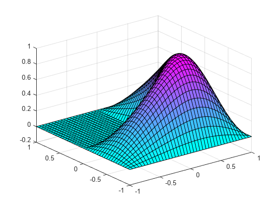
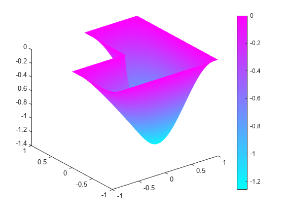
Compute the sixteenth eigenvalue, and plot the sixteenth eigenmode.
l(16) % sixteenth eigenvalue
ans = 92.5224
figure pdeplot(model,'XYData',v(:,16),'ZData',v(:,16)) % sixteenth eigenmode
Eigenvalues and Eigenvectors of the L-Shaped Membrane Using Legacy Syntax
Compute the eigenvalues that are less than 100, and compute the corresponding eigenmodes for on the geometry of the L-shaped membrane, using the legacy syntax.
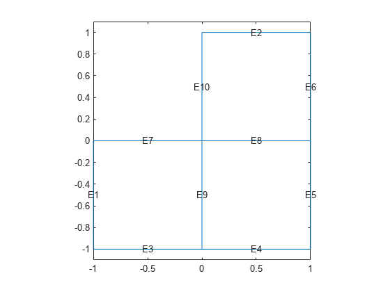
Use the geometry in lshapeg
. For more information about this syntax, see Parametrized Function for 2-D Geometry Creation.
g = @lshapeg; pdegplot(g,'EdgeLabels','on') axis equal ylim([-1.1,1.1])
Set zero Dirichlet boundary conditions using the lshapeb
function.
b = @lshapeb;
Set coefficients c = 1
, a = 0
, and d = 1
. Collect eigenvalues up to 100.
c = 1; a = 0; d = 1; r = [-Inf 100];
Generate a mesh and solve the eigenvalue problem.
[p,e,t] = initmesh(g,'Hmax',0.02);
[v,l] = pdeeig(b,p,e,t,c,a,d,r);
Find the first eigenvalue.
l(1)
ans = 9.6481
Eigenvalues and Eigenvectors Using Finite Element Matrices
Import a simple 3-D geometry and find eigenvalues and eigenvectors from the associated finite element matrices.
Create a model and import the BracketWithHole.stl
geometry.
model = createpde(); importGeometry(model,'BracketWithHole.stl'); figure pdegplot(model,'FaceLabels','on') view(30,30) title('Bracket with Face Labels')
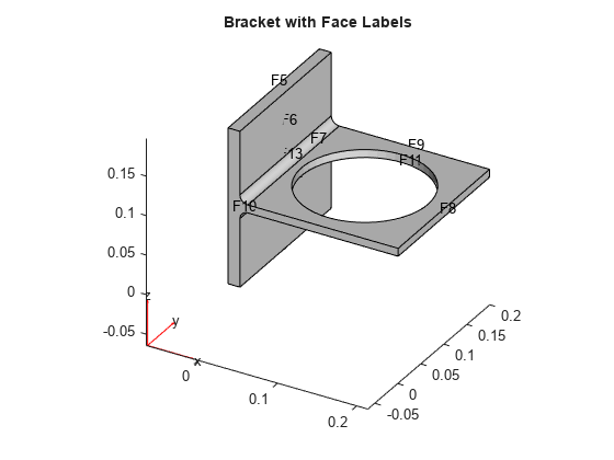
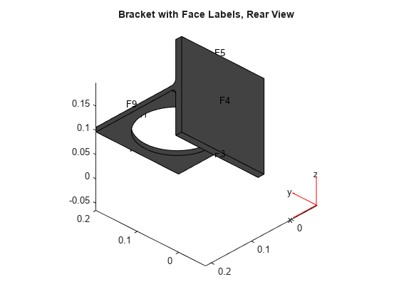
figure pdegplot(model,'FaceLabels','on') view(-134,-32) title('Bracket with Face Labels, Rear View')
Set coefficients c = 1
, a = 0
, and d = 1
. Collect eigenvalues that are less than 100.
c = 1; a = 0; d = 1; r = [-Inf 100];
Generate a mesh for the model.
generateMesh(model);
Create the associated finite element matrices.
[Kc,~,B,~] = assempde(model,c,a,0); [~,M,~] = assema(model,0,d,0);
Solve the eigenvalue problem.
[v,l] = pdeeig(Kc,B,M,r);
Look at the first two eigenvalues.
l([1,2])
ans = 2×1
-0.0000
42.8014
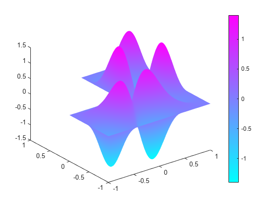
Plot the solution corresponding to eigenvalue 2.
pdeplot3D(model,'ColorMapData',v(:,2))
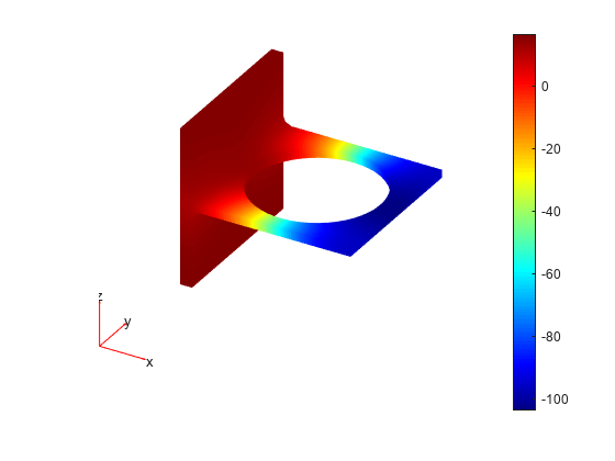
Input Arguments
model
— PDE model
PDEModel
object
PDE model, specified as a PDEModel
object.
Example: model = createpde
c
— PDE coefficient
scalar | matrix | character vector | character array | string scalar | string vector | coefficient function
PDE coefficient, specified as a scalar, matrix, character vector,
character array, string scalar, string vector, or coefficient function.
c
represents the c coefficient in
the scalar PDE
or the system PDE eigenvalue problem
Example: 'cosh(x+y.^2)'
Data Types: double
| char
| string
| function_handle
Complex Number Support: Yes
a
— PDE coefficient
scalar | matrix | character vector | character array | string scalar | string vector | coefficient function
PDE coefficient, specified as a scalar, matrix, character vector,
character array, string scalar, string vector, or coefficient function.
a
represents the a coefficient in
the scalar PDE
or the system PDE eigenvalue problem
Example: 2*eye(3)
Data Types: double
| char
| string
| function_handle
Complex Number Support: Yes
d
— PDE coefficient
scalar | matrix | character vector | character array | string scalar | string vector | coefficient function
PDE coefficient, specified as a scalar, matrix, character vector,
character array, string scalar, string vector, or coefficient function.
d
represents the d coefficient in
the scalar PDE
or the system PDE eigenvalue problem
Example: 2*eye(3)
Data Types: double
| char
| string
| function_handle
Complex Number Support: Yes
r
— Eigenvalue range
two-element real vector
Eigenvalue range, specified as a two-element real vector. Real parts of
eigenvalues λ fall in the range
r(1)
≤ λ ≤ r(2)
.
r(1)
can be -Inf
. The algorithm
returns all eigenvalues in this interval in the l
output, up to a maximum of 99 eigenvalues.
Example: [-Inf,100]
Data Types: double
b
— Boundary conditions
boundary matrix | boundary file
Boundary conditions, specified as a boundary matrix or boundary file. Pass a boundary file as a function handle or as a file name. A boundary matrix is generally an export from the PDE Modeler app.
Example: b = 'circleb1'
, b = "circleb1"
, or b =
@circleb1
Data Types: double
| char
| string
| function_handle
p
— Mesh points
matrix
Mesh points, specified as a 2-by-Np
matrix of points, where
Np
is the number of points in the mesh. For a description of the
(p
,e
,t
) matrices, see Mesh Data as [p,e,t] Triples.
Typically, you use the p
, e
, and t
data exported from the PDE Modeler app, or generated by initmesh
or refinemesh
.
Example: [p,e,t] = initmesh(gd)
Data Types: double
e
— Mesh edges
matrix
Mesh edges, specified as a 7
-by-Ne
matrix of edges,
where Ne
is the number of edges in the mesh. For a description of the
(p
,e
,t
) matrices, see Mesh Data as [p,e,t] Triples.
Typically, you use the p
, e
, and t
data exported from the PDE Modeler app, or generated by initmesh
or refinemesh
.
Example: [p,e,t] = initmesh(gd)
Data Types: double
t
— Mesh triangles
matrix
Mesh triangles, specified as a 4
-by-Nt
matrix of
triangles, where Nt
is the number of triangles in the mesh. For a
description of the (p
,e
,t
)
matrices, see Mesh Data as [p,e,t] Triples.
Typically, you use the p
, e
, and t
data exported from the PDE Modeler app, or generated by initmesh
or refinemesh
.
Example: [p,e,t] = initmesh(gd)
Data Types: double
Kc
— Stiffness matrix
sparse matrix | full matrix
Stiffness matrix, specified as a sparse matrix or as a full
matrix. See Elliptic Equations. Typically, Kc
is
the output of assempde
.
B
— Dirichlet nullspace
sparse matrix
Dirichlet nullspace, returned as a sparse matrix. See Algorithms. Typically, B
is
the output of assempde
.
M
— Mass matrix
sparse matrix | full matrix
Mass matrix. specified as a sparse matrix or a full matrix. See Elliptic Equations.
To obtain the input matrices for pdeeig
, hyperbolic
or parabolic
,
run both assema
and assempde
:
[Kc,Fc,B,ud] = assempde(model,c,a,f); [~,M,~] = assema(model,0,d,f);
Note
Create the M
matrix using assema
with d
,
not a
, as the argument before f
.
Data Types: double
Complex Number Support: Yes
Output Arguments
v
— Eigenvectors
matrix
Eigenvectors, returned as a matrix. Suppose
Np
is the number of mesh nodesN is the number of equations
ev
is the number of eigenvalues returned inl
Then v
has size
Np
*N-by-ev
.
Each column of v
corresponds to the eigenvectors of one
eigenvalue. In each column, the first Np
elements
correspond to the eigenvector of equation 1 evaluated at the mesh nodes, the
next Np
elements correspond to equation 2, etc.
Note
Eigenvectors are determined only up to multiple by a scalar, including a negative scalar.
l
— Eigenvalues
vector
Eigenvalues, returned as a vector. The real parts of l
are in the interval r
. The real parts of
l
are monotone increasing.
Limitations
In the standard case c and d are positive in the entire region. All eigenvalues are positive, and 0 is a good choice for a lower bound of the interval. The cases where either c or d is zero are discussed next.
If d = 0 in a subregion, the mass matrix M becomes singular. This does not cause any trouble, provided that c > 0 everywhere. The pencil (K,M) has a set of infinite eigenvalues.
If c = 0 in a subregion, the stiffness matrix
K
becomes singular, and the pencil (K,M) has many zero eigenvalues. With an interval containing zero,pdeeig
goes on for a very long time to find all the zero eigenvalues. Choose a positive lower bound away from zero but below the smallest nonzero eigenvalue.If there is a region where both c = 0 and d = 0, we get a singular pencil. The whole eigenvalue problem is undetermined, and any value is equally plausible as an eigenvalue.
Some of the awkward cases are detected by pdeeig
. If the shifted
matrix is singular, another shift is attempted. If the matrix with the new shift is
still singular a good guess is that the entire pencil (K,M) is
singular.
If you try any problem not belonging to the standard case, you must use your knowledge of the original physical problem to interpret the results from the computation.
Tips
The equation coefficients cannot depend on the solution
u
or its gradient.
Algorithms
Eigenvalue Equations
Partial Differential Equation Toolbox™ software handles the following basic eigenvalue problem:
where λ is an unknown complex number. In solid mechanics, this is a problem associated with wave phenomena describing, e.g., the natural modes of a vibrating membrane. In quantum mechanics λ is the energy level of a bound state in the potential well a(x), where x represents a 2-D or 3-D point.
The numerical solution is found by discretizing the equation and solving the resulting algebraic eigenvalue problem. Let us first consider the discretization. Expand u in the FEM basis, multiply with a basis element, and integrate on the domain Ω. This yields the generalized eigenvalue equation
KU = λMU
where the mass matrix corresponds to the right side, i.e.,
The matrices K and M are produced by calling
assema
for the equations
–∇ · (c∇u) + au = 0 and –∇ · (0∇u) + du = 0
In the most common case, when the function d(x) is positive, the mass matrix M is positive definite symmetric. Likewise, when c(x) is positive and we have Dirichlet boundary conditions, the stiffness matrix K is also positive definite.
The generalized eigenvalue problem, KU = λMU, is now solved by the Arnoldi algorithm applied to a shifted and inverted matrix with restarts until all eigenvalues in the user-specified interval have been found.
Let us describe how this is done in more detail. You may want to look at the examples Eigenvalues and Eigenmodes of L-Shaped Membrane or Eigenvalues and Eigenmodes of Square, where actual runs are reported.
First a shift µ is determined close to where we want to find the eigenvalues. When both K and M are positive definite, it is natural to take µ = 0, and get the smallest eigenvalues; in other cases take any point in the interval [lb,ub] where eigenvalues are sought. Subtract µM from the eigenvalue equation and get (K - µM)U = (λ - µ)MU. Then multiply with the inverse of this shifted matrix and get
This is a standard eigenvalue problem AU = θU, with the matrix A = (K – µM)-1M and eigenvalues
where i = 1, . . ., n. The largest eigenvalues θi of the transformed matrix A now correspond to the eigenvalues λi = µ + 1/θi of the original pencil (K,M) closest to the shift µ.
The Arnoldi algorithm computes an orthonormal basis V where the shifted and inverted operator A is represented by a Hessenberg matrix H,
AVj = VjHj,j + Ej.
(The subscripts mean that Vj and Ej have j columns and Hj,j has j rows and columns. When no subscripts are used we deal with vectors and matrices of size n.)
Some of the eigenvalues of this Hessenberg matrix Hj,j eventually give good approximations to the eigenvalues of the original pencil (K,M) when the basis grows in dimension j, and less and less of the eigenvector is hidden in the residual matrix Ej.
The basis V is built one column vj at a time. The first vector v1 is chosen at random, as n normally distributed random numbers. In step j, the first j vectors are already computed and form the n ×j matrix Vj. The next vector vj+1 is computed by first letting A operate on the newest vector vj, and then making the result orthogonal to all the previous vectors.
This is formulated as , where the column vector hj consists of the Gram-Schmidt coefficients, and hj+1,j is the normalization factor that gives vj+1 unit length. Put the corresponding relations from previous steps in front of this and get
where Hj,j is a j×j Hessenberg matrix with the vectors hj as columns. The second term on the right-hand side has nonzeros only in the last column; the earlier normalization factors show up in the subdiagonal of Hj,j.
The eigensolution of the small Hessenberg matrix H gives approximations to some of the eigenvalues and eigenvectors of the large matrix operator Aj,j in the following way. Compute eigenvalues θi and eigenvectors si of Hj,j,
Then yi = Vjsi is an approximate eigenvector of A, and its residual is
This residual has to be small in norm for θi to be a good eigenvalue approximation. The norm of the residual is
the product of the last subdiagonal element of the Hessenberg matrix and the last element of its eigenvector. It seldom happens that hj+1,j gets particularly small, but after sufficiently many steps j there are always some eigenvectors si with small last elements. The long vector Vj+1 is of unit norm.
It is not necessary to actually compute the eigenvector approximation yi to get the norm of the residual; we only need to examine the short vectors si, and flag those with tiny last components as converged. In a typical case n may be 2000, while j seldom exceeds 50, so all computations that involve only matrices and vectors of size j are much cheaper than those involving vectors of length n.
This eigenvalue computation and test for convergence is done every few steps j, until all approximations to eigenvalues inside the interval [lb,ub] are flagged as converged. When n is much larger than j, this is done very often, for smaller n more seldom. When all eigenvalues inside the interval have converged, or when j has reached a prescribed maximum, the converged eigenvectors, or more appropriately Schur vectors, are computed and put in the front of the basis V.
After this, the Arnoldi algorithm is restarted with a random vector, if all approximations inside the interval are flagged as converged, or else with the best unconverged approximate eigenvector yi. In each step j of this second Arnoldi run, the vector is made orthogonal to all vectors in V including the converged Schur vectors from the previous runs. This way, the algorithm is applied to a projected matrix, and picks up a second copy of any double eigenvalue there may be in the interval. If anything in the interval converges during this second run, a third is attempted and so on, until no more approximate eigenvalues θi show up inside. Then the algorithm signals convergence. If there are still unconverged approximate eigenvalues after a prescribed maximum number of steps, the algorithm signals nonconvergence and reports all solutions it has found.
This is a heuristic strategy that has worked well on both symmetric, nonsymmetric, and even defective eigenvalue problems. There is a tiny theoretical chance of missing an eigenvalue, if all the random starting vectors happen to be orthogonal to its eigenvector. Normally, the algorithm restarts p times, if the maximum multiplicity of an eigenvalue is p. At each restart a new random starting direction is introduced.
The shifted and inverted matrix A = (K – µM)–1M is needed only to operate on a vector vj in the Arnoldi algorithm. This is done by computing an LU factorization,
P(K – µM)Q = LU
using the sparse MATLAB® command lu
(P and Q
are permutations that make the triangular factors L and
U sparse and the factorization numerically stable). This
factorization needs to be done only once, in the beginning, then x =
Avj is computed as,
x = QU–1L–1PMvj
with one sparse matrix vector multiplication, a permutation, sparse forward- and back-substitutions, and a final renumbering.
Version History
Introduced before R2006aR2016a: Not recommended
pdeeig
is not recommended. Use solvepdeeig
instead. There are no plans to remove
pdeeig
.
See Also
Comando MATLAB
Hai fatto clic su un collegamento che corrisponde a questo comando MATLAB:
Esegui il comando inserendolo nella finestra di comando MATLAB. I browser web non supportano i comandi MATLAB.
Select a Web Site
Choose a web site to get translated content where available and see local events and offers. Based on your location, we recommend that you select: .
You can also select a web site from the following list:
How to Get Best Site Performance
Select the China site (in Chinese or English) for best site performance. Other MathWorks country sites are not optimized for visits from your location.
Americas
- América Latina (Español)
- Canada (English)
- United States (English)
Europe
- Belgium (English)
- Denmark (English)
- Deutschland (Deutsch)
- España (Español)
- Finland (English)
- France (Français)
- Ireland (English)
- Italia (Italiano)
- Luxembourg (English)
- Netherlands (English)
- Norway (English)
- Österreich (Deutsch)
- Portugal (English)
- Sweden (English)
- Switzerland
- United Kingdom (English)