Stiff Differential Equations
By Cleve Moler, MathWorks
Stiffness is a subtle, difficult, and important - concept in the numerical solution of ordinary differential equations.
It depends on the differential equation, the initial conditions, and the numerical method. Dictionary definitions of the word " stiff" involve terms like "not easily bent," "rigid," and "stubborn." We are concerned with a computational version of these properties.
An ordinary differential equation problem is stiff if the solution being sought is varying slowly, but there are nearby solutions that vary rapidly, so the numerical method must take small steps to obtain satisfactory results.
Stiffness is an efficiency issue. If we weren't concerned with how much time a computation takes, we wouldn't be concerned about stiffness. Nonstiff methods can solve stiff problems; they just take a long time to do it.
A model of flame propagation provides an example. We learned about this example from Larry Shampine, one of the authors of the MATLAB ODE suite. When you light a match, the ball of flame grows rapidly until it reaches a critical size. Then it remains at that size because the amount of oxygen being consumed by the combustion in the interior of the ball balances the amount available through the surface. The simple model is
\[\begin{align}\frac{dy}{dt} &= y^2 - y^3\\ y(0) &=\delta \\ 0 &< t < \frac{2}{\delta}\end{align}\]
The scalar variable \(y(t)\) represents the radius of the ball. The \(y^2\)and \(y^3\) terms come from the surface area and the volume. The critical parameter is the initial radius, \(\delta\), which is "small." We seek the solution over a length of time that is inversely proportional to \(\delta\).
At this point, we suggest that you start up MATLAB and actually run our examples. It is worthwhile to see them in action. We will start with ode45, the workhorse of the MATLAB ODE suite. If \(\delta\) is not very small, the problem is not very stiff. Try \(\delta = 0.01\) and request a relative error of \(10^{-4}\).
delta = 0.01;
F = inline('y^2 - y^3','t','y');
opts = odeset('RelTol',1.e-4);
ode45(F,[0 2/delta],delta,opts);
With no output arguments, ode45 automatically plots the solution as it is computed. You should get a plot of a solution that starts at \(y = .01\), grows at a modestly increasing rate until \(t\) approaches 50, which is \(1/\delta\), then grows rapidly until it reaches a value close to 1, where it remains.
Now let's see stiffness in action. Decrease \(\delta\) by a couple of orders of magnitude. (If you run only one example, run this one.)
delta = 0.0001;
ode45(F,[0 2/delta],delta,opts);
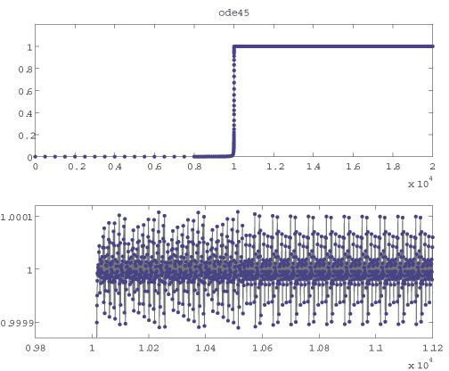
You should see something like our first figure, although it will take a long time to complete the plot. If you get tired of watching the agonizing progress, click the stop button in the lower-left corner of the window. Turn on zoom, and use the mouse to explore the solution near where it first reaches steady state. You should see something like the detail in the first figure. Notice that ode45 is doing its job. It's keeping the solution within \(10^{-4}\) of its nearly constant steady-state value. But it certainly has to work hard to do it. If you want an even more dramatic demonstration of stiffness, decrease the tolerance to \(10^{-5}\) or \(10^{-6}\).
This problem is not stiff initially. It only becomes stiff as the solution approaches steady state. This is because the steady-state solution is so "rigid." Any solution near \(y(t) = 1\) increases or decreases rapidly toward that solution. We should point out that "rapidly" here is with respect to an unusually long time scale.
What can be done about stiff problems? You don't want to change the differential equation or the initial conditions, so you have to change the numerical method. Methods intended to solve stiff problems efficiently do more work per step, but can take much bigger steps. Stiff methods are implicit. At each step they use MATLAB matrix operations to solve a system of simultaneous linear equations that helps predict the evolution of the solution. For our flame example, the matrix is only 1 by 1, but even here, stiff methods do more work per step than nonstiff methods.
Let's compute the solution to our flame example again, this time with one of the ODE solvers in MATLAB whose name ends in "s" for "stiff."
delta = 0.0001;
ode23s(F,[0 2/delta],delta,opts);
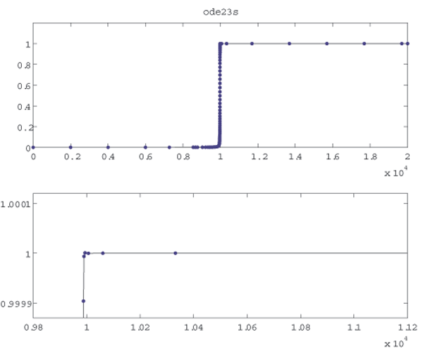
The second figure shows the computed solution and the zoom detail. You can see that ode23s takes many fewer steps than ode45. This is actually an easy problem for a stiff solver. In fact, ode23s takes only 99 steps and uses just 412 function evaluations, while ode45 takes 3,040 steps and uses 20,179 function evaluations. Stiffness even affects graphical output. Our print files for the ode45 figures are much larger than those for the ode23s figures.
Imagine you are returning from a hike in the mountains. You are in a narrow canyon with steep walls on either side. An explicit algorithm would sample the local gradient to find the descent direction. But following the gradient on either side of the trail will send you bouncing back and forth from wall to wall, as in Figure 1. You will eventually get home, but it will be long after dark before you arrive. An implicit algorithm would have you keep your eyes on the trail and anticipate where each step is taking you. It is well worth the extra concentration.
This flame problem is also interesting because it involves something called the Lambert W function, \(W(z)\). The differential equation is separable. Integrating once gives an implicit equation for \(y\) as a function of \(t\).
\[\frac{1}{y} + \log\left(\frac{1}{y}-1\right) = \frac{1}{\delta} + \log\left(\frac{1}{\delta} - 1\right) - t\]
This equation can be solved for y. The exact analytical solution to the flame model turns out to be
\[y(t) = \frac{1}{(W(a e^{a - t}) + 1)}\]
where \(a = \frac{1}{\delta} - 1\). The function \(W(z)\), the Lambert W function, is the solution to
\[W(z)e^{W(z)} = z\]
With MATLAB and the Symbolic Math Toolbox connection to Maple, the statements
y = dsolve('Dy = y^2 - y^3','y(0) = 1/100');
y = simplify(y);
pretty(y)
ezplot(y,0,200)
produce
                  1
---------------------------------------
lambertw(99 exp(99 - t)) + 1
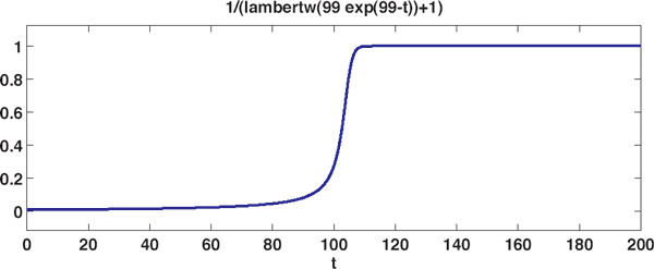
and a plot of the exact solution. When the initial value, 1/100, is decreased, and the time span \(0 \leq t \leq 200\) is increased, the transition region becomes narrower.
The Lambert W function is named after J. H. Lambert (1728 - 1777), who was a colleague of Euler and Lagrange at the Berlin Academy of Sciences. Lambert is best known for his laws of illumination and his proof that π is irrational. The function was "rediscovered" a few years ago by Corless, Gonnet, Hare, and Jeffrey, working on Maple, and by Don Knuth. The existence of an exact solution to this nonlinear problem allows us to rigorously assess the accuracy of both the stiff and nonstiff numerical methods.
Published 2003
References
-
Robert M. Corless, G. H. Gonnet, D. E. G. Hare, D. J. Jeffrey, and D. E. Knuth, “ On the Lambert W Function,” Advances in Computational Mathematics, Volume 5, 1996, pp. 329-359.


