Interact with Polar Plot
This example shows how to interact with a polar plot created using polarpattern object.
Create Polar Plot of Helix Antenna
Create a helix antenna with a 28 mm radius, 1.2 mm width and 4 turns.
hx = helix(Radius=28e-3,Width=1.2e-3,Turns=4);
Calculate the elevation cut of the antenna directivity at 1.8 GHz.
H = pattern(hx,1.8e9,0,0:1:360);
View the polar plot of the antenna directivity.
P0 = polarpattern(H);

Interact with Polar Plot
Hover over the plot. You see a message on top of the plot: Right click to interact with the plot. Right-click anywhere in the Polar Measurement window to display a context menu for interacting with the plot. For example, right-click outside the plot to show the Main context menu. Right-click inside the plot to show the Display context menu.

Update Angle and Magnitude Values
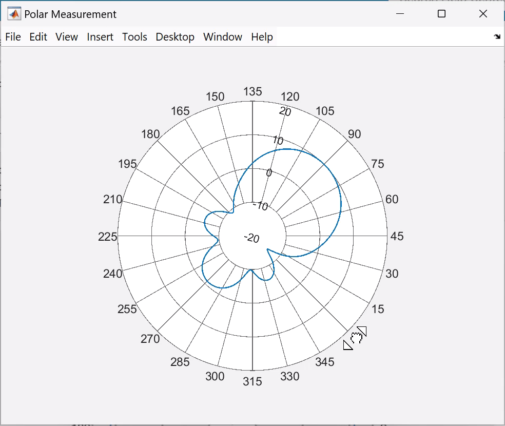
The angular values are around the circumference of the polar plot. Right-click any of the angle values to open ANGLE context menu. By default, the angles are displayed CCW (counterclockwise).
Change the resolution from 15 degrees to 10 degrees.

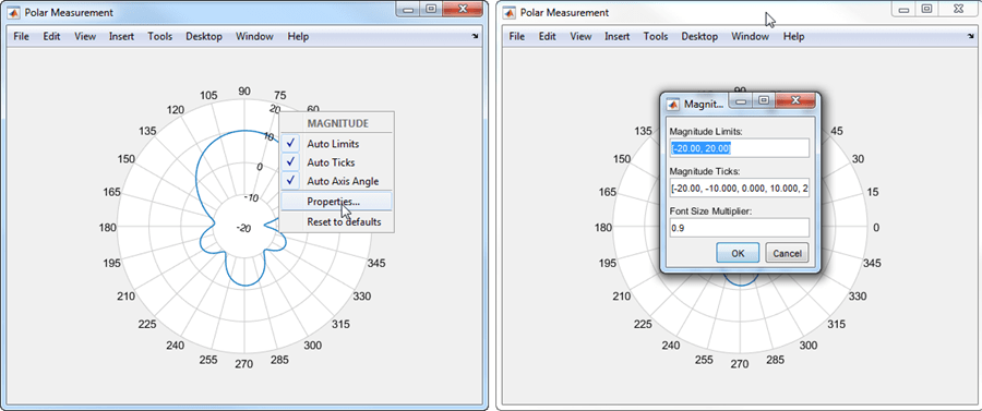
The magnitude values are on the radial lines of the plot. Right-click any of the magnitude values to open the MAGNITUDE context menu. Choose properties from the context menu to change the magnitude limits, magnitude ticks, or font size.
Add Cursors and Calculate Angle Span
Add cursors at 60 degrees and 105 degrees.
To add a cursor from the MAIN or DISPLAY context menus, select Measurements > Add Cursor. After adding the cursor, place the mouse pointer on the cursor and drag it to 60 degrees.

You can also add a cursor by double-clicking on the angle values. Double-click 105 to add a cursor. Right-click the newly added cursor and move the cursor to exact value of 105 degrees.
You can also interpolate the two angle values to 60 degrees and 150 degrees. Right-click on each cursor and choose Interpolate from the CURSOR context menu. To set the angle span, from the MAIN or DISPLAY context menu, select Measurements > Angle Span.

Calculate the counterclockwise angle span between 60 degrees and 105 degrees.

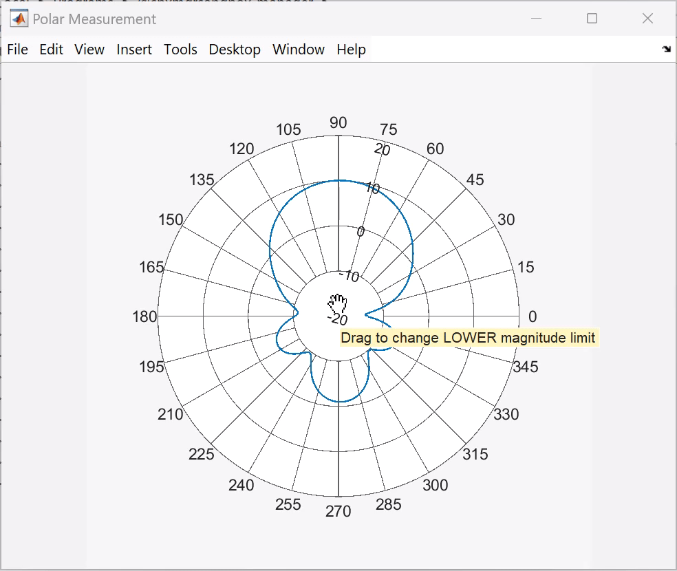
Change Lower Limit of Magnitude Scale
You can click on the lowest magnitude value on the plot and drag the mouse pointer radially outward to change it.
Zoom In and Zoom Out
Move the mouse pointer on the plot and scroll to zoom in or zoom out of the plot.


Rotate Plot
Click on any angle value and drag the mouse clockwise or anticlockwise to rotate the plot.

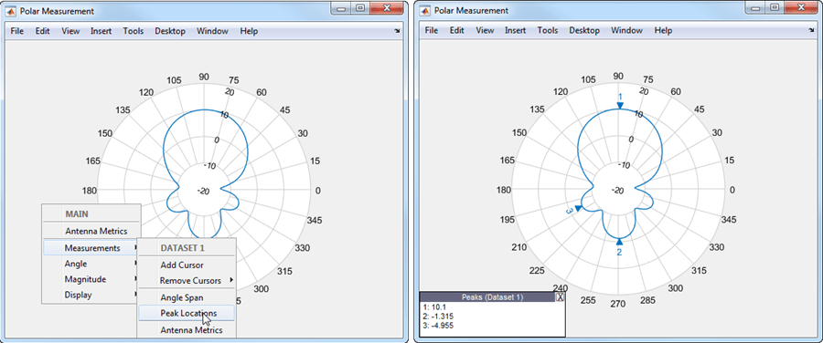
Display Peak Locations
To display the peak locations from the MAIN or DISPLAY context menus, select Measurements > Peak Location.

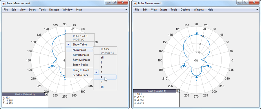
Right-click any of the peak triangles and choose NumPeaks. Increase the number of peaks to 4.
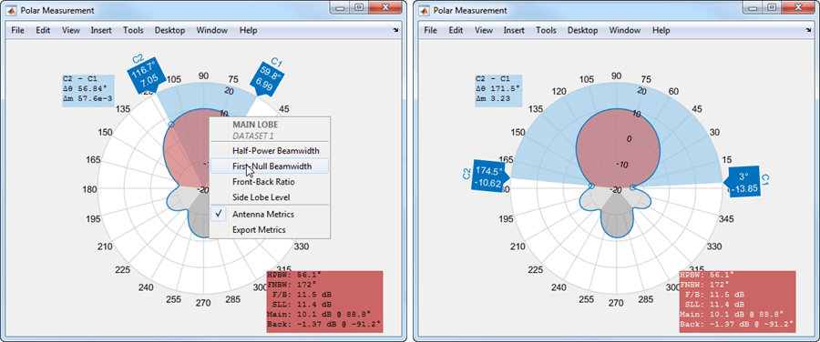
View Antenna Metrics
Antenna metrics in the polar plot display the main, back, and side lobes of the antenna. There are two ways to turn display antenna metrics on the plot:
1. Right-click within the polar figure to open the Main context menu. Choose Antenna Metrics.
2. Right-click inside the polar plot to open the Display context menu. Inside the Measurement menu, choose Antenna Metrics.
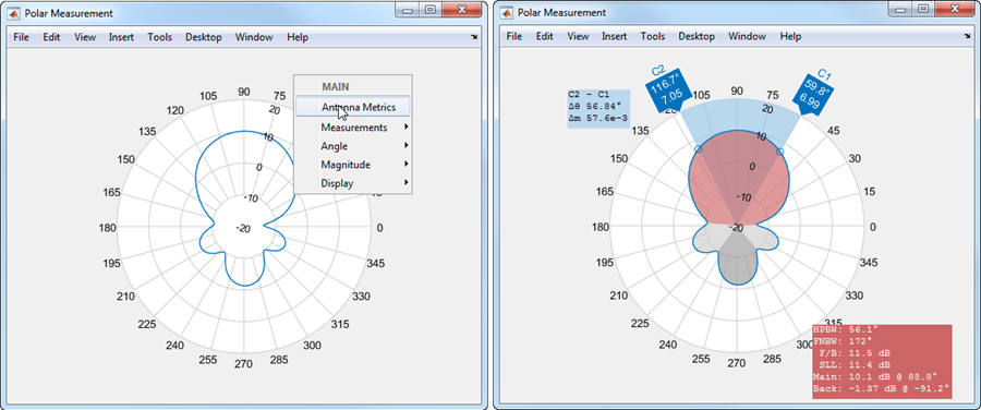
By default, the plot shows the HPBW (half-power beamwidth) of the antenna. The antenna measurements text box displays:
HPBW(half-power beamwidth)FNBW(first-null beamwidth)F/B(front-to-back ratio)SLL(side lobe level)Main(main lobe peak value and corresponding angle)Back(back lobe peak value and corresponding angle)
To view the FNBW, right-click inside the red or gray polar plot region to open the MAIN LOBE or the BACK LOBE context menu and then choose First-Null Beamwidth.
Hide Specific Region of Plot
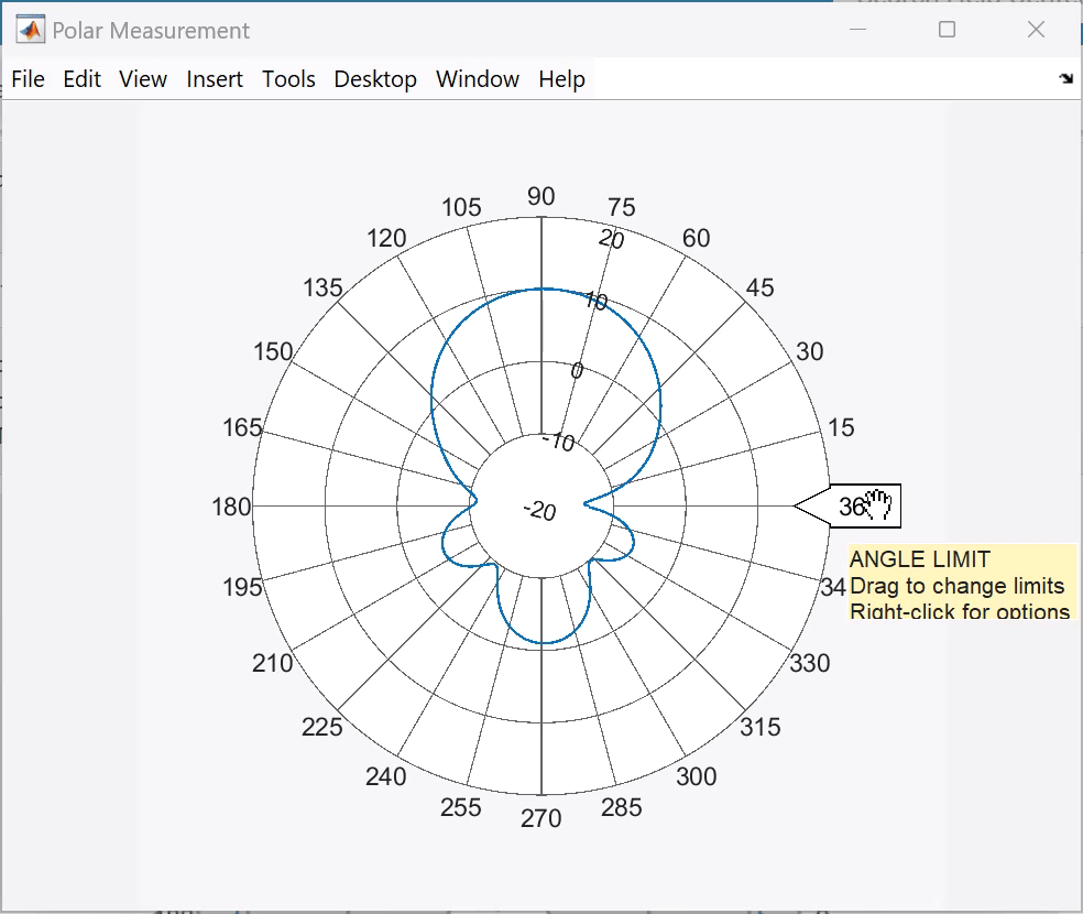
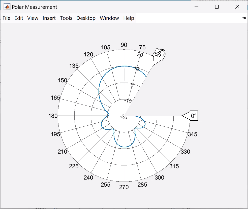
Set the AngleLimVisible property to 1 to display the angle labels.
P1 = polarpattern(H,AngleLimVisible=1);
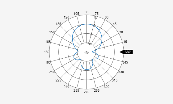
Click and rotate the angle label to specify a range of angles on the plot to hide the region between these angles.