Compare Conditional Variance Model Fit Statistics Using Econometric Modeler App

This example shows how to specify and fit GARCH, EGARCH, and GJR models to data using the Econometric Modeler app. Then, the example determines the model that fits to the data the best by comparing fit statistics. The data set, which is stored in Data_FXRates.mat, contains foreign exchange rates measured daily from 1979–1998.

Consider creating a predictive model for the Swiss franc to US dollar exchange rate (CHF).

Import Data into Econometric Modeler

At the command line, load the Data_FXRates.mat data set.

load Data_FXRates

At the command line, open the Econometric Modeler app.

econometricModeler

Alternatively, open the app from the apps gallery (see Econometric Modeler).

Import DataTimeTable into the app:

1. On the Modeler tab, in the Import section, click the Import button .

2. In the Import Data dialog box, select the check box for the DataTimeTable variable.

3. Click Import.

All time series variables in DataTimeTable appear in the Time Series pane, and a time series plot of all the series appears in the Plot(AUD) figure window.

Plot the Series

Plot the Swiss franc exchange rates by double-clicking the CHF time series in the Time Series pane.

Highlight periods of recession:

1. In the Plot(CHF) figure window, right-click the plot.

2. In the context menu, select Show Recessions.

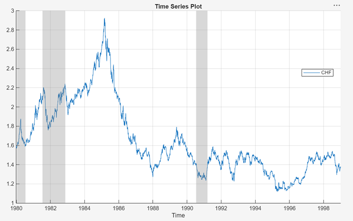
The CHF series appears to have a stochastic trend.

Stabilize the Series

Stabilize the Swiss franc exchange rates by applying the first difference to CHF.

1. In the Time Series pane, select CHF.

2. On the Modeler tab, in the Transforms section, click Difference.

A variable named CHF_Diff, representing the differenced series, appears in the Time Series pane, its value appears in the Preview pane, and its time series plot appears in the Plot(CHF_Diff) figure window.

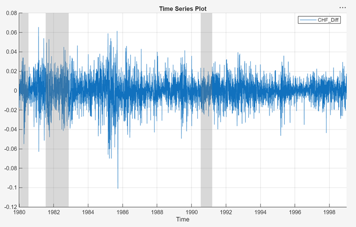
The series appears to be stable, but it exhibits volatility clustering.

Assess Presence of Conditional Heteroscedasticity

Test the stable Swiss franc exchange rate series for conditional heteroscedasticity by conducting Engle's ARCH test. Run the test assuming an ARCH(1) alternative model, then run the test again assuming an ARCH(2) alternative model. Maintain an overall significance level of 0.05 by decreasing the significance level of each test to 0.05/2 = 0.025.

1. In the Time Series pane, select CHF_Diff.

2. On the Modeler tab, in the Tests section, click Add Test > Engle's ARCH Test.

3. On the ARCH tab, in the Settings section, set Number of Lags of 1.

4. Set Significance Level to 0.025.

5. In the Tests section, click Run Test.

6. Repeat steps 3 through 5, but set Number of Lags to 2 instead.

The test results appear in the Results table of the ARCH(CHF_Diff) document.

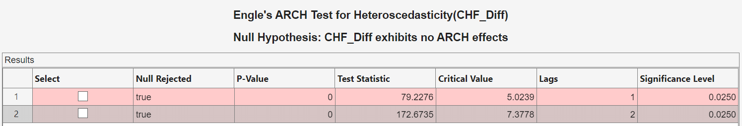
The tests reject the null hypothesis of no ARCH effects against the alternative models. This result suggests specifying a conditional variance model for CHF_Diff containing at least two ARCH lags. Conditional variance models with two ARCH lags are locally equivalent to models with one ARCH and one GARCH lag. Consider GARCH(1,1), EGARCH(1,1), and GJR(1,1) models for CHF_Diff.

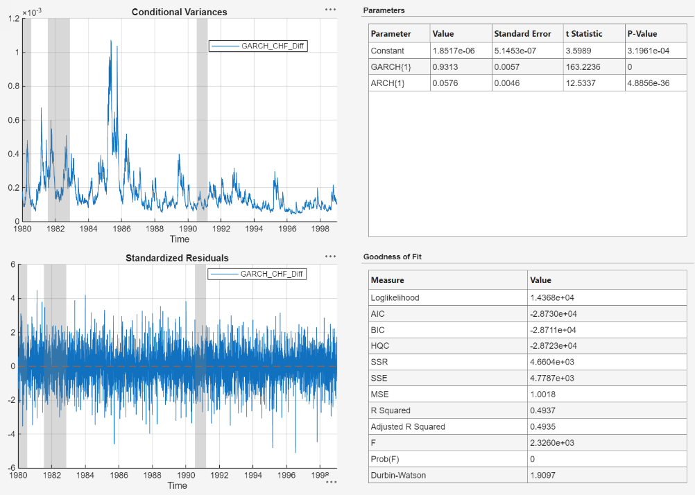
Estimate GARCH Model

Specify a GARCH(1,1) model and fit it to the CHF_Diff series.

1. In the Time Series pane, select the CHF_Diff time series.

2. Click the Modeler tab. Then, in the Models section, click the arrow to display the models gallery.

3. In the models gallery, in the GARCH Models section, click GARCH.

4. In the GARCH Model Parameters dialog box, on the Lag Order tab, clear the Include Offset check box, then click Estimate.

   

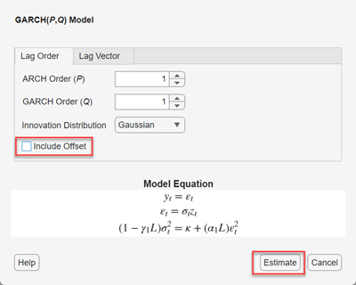
The model variable GARCH_CHF_Diff appears in the Models pane, its value appears in the Preview pane, and its estimation summary appears in the Fit(GARCH_CHF_Diff) document.

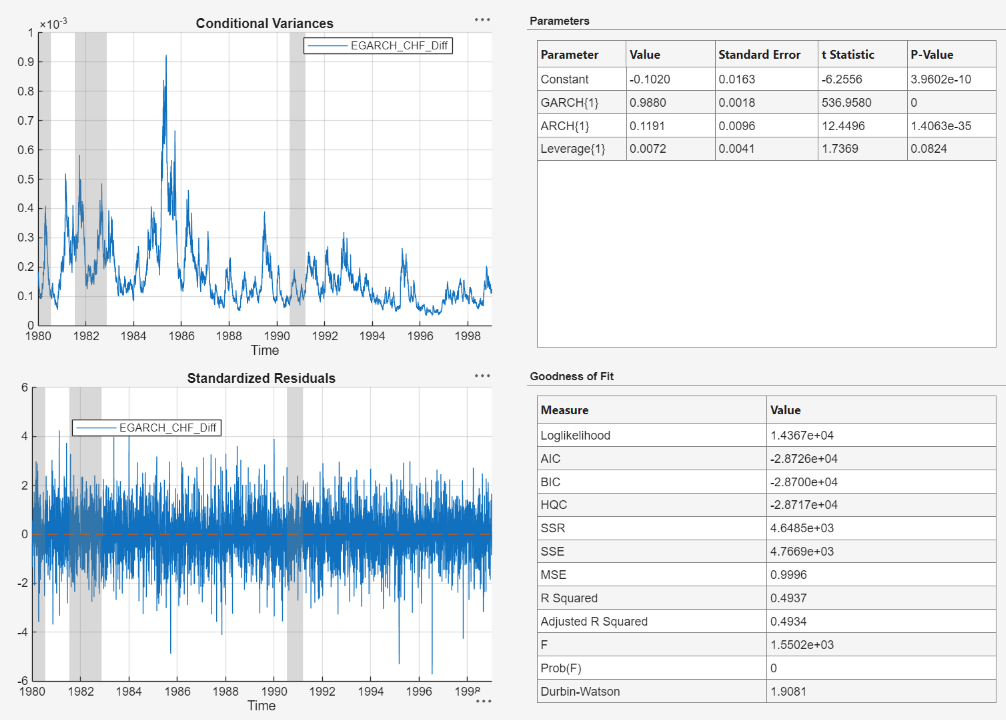
Specify and Estimate EGARCH Model

Specify an EGARCH(1,1) model containing a leverage term at the first lag, and fit the model to the CHF_Diff series.

1. In the Time Series pane, select the CHF_Diff time series.

2. On the Modeler tab, in the Models section, click the arrow to display the models gallery.

3. In the models gallery, in the GARCH Models section, click EGARCH.

4. In the EGARCH Model Parameters dialog box, on the Lag Order tab, clear the Include Offset check box, then click Estimate.

   Econometric Modeler includes a leverage lag for each ARCH lag. You can remove or adjust leverage lags on the Lag Vector tab.

The model variable EGARCH_CHF_Diff appears in the Models pane, its value appears in the Preview pane, and its estimation summary appears in the Fit(EGARCH_CHF_Diff) document.

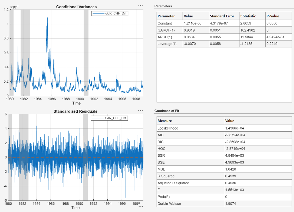
Specify and Estimate GJR Model

Specify a GJR(1,1) model containing a leverage term at the first lag, and fit the model to the CHF_Diff series.

1. In the Time Series pane, select the CHF_Diff time series.

2. On the Modeler tab, in the Models section, click the arrow to display the models gallery.

3. In the models gallery, in the GARCH Models section, click GJR.

4. In the GJR Model Parameters dialog box, on the Lag Order tab, clear the Include Offset check box, then click Estimate.

   Econometric Modeler includes a leverage lag for each ARCH lag. You can remove or adjust leverage lags on the Lag Vector tab.

The model variable GJR_CHF_Diff appears in the Models pane, its value appears in the Preview pane, and its estimation summary appears in the Fit(GJR_CHF_Diff) document.

Choose Model

Choose the model with the best parsimonious in-sample fit. Base your decision on the model yielding the minimal Akaike information criterion (AIC). The table shows the AIC fit statistics of the estimated models, as given in the Goodness of Fit section of the estimation summary of each model.

Model	AIC
GARCH(1,1)	-28730
EGARCH(1,1)	-28726
GJR(1,1)	-28724

The GARCH(1,1) model yields the minimal AIC value. Therefore, it has the best parsimonious in-sample fit of all the estimated models.