Find Manufacturing Tolerances Using Inverse Sensitivity Analysis

R2026b

Since R2026b

This example demonstrates how to determine the maximum allowable manufacturing tolerances for an optical system using inverse sensitivity analysis. Given a target image quality specification, inverse sensitivity finds the largest tolerance for each parameter that keeps the total error within budget. Use inverse sensitivity analysis to determine what tolerance values to provide on the manufacturing drawing during fabrication.

In this example, you perform these steps.

1. Run forward sensitivity analysis to identify which parameters are most sensitive.

2. Use bisection search with iterative Root Sum Squared (RSS) budget reallocation to find the maximum allowable tolerance for each parameter.

3. Verify that the found tolerances meet the specification.

This example requires the Optical Design and Simulation Library for Image Processing Toolbox™ and the Optimization Toolbox™. The compensator uses the Optimization Toolbox during sensitivity analysis to optimize the position of the image plane. You can install the Optical Design and Simulation Library for Image Processing Toolbox from the Add-On Explorer. For more information about installing add-ons, see Get and Manage Add-Ons.

If the Parallel Computing Toolbox™ is available, sensitivity evaluations run in parallel on a local cluster for faster execution. Without the Parallel Computing Toolbox, the sensitivity evaluations run sequentially.

Import Cooke Triplet

The five Seidel aberrations are the primary defects that degrade image quality in optical systems. Specifically, the Seidel aberrations are spherical aberration, coma, astigmatism, field curvature, and distortion. The Cooke triplet is a three-element lens design that corrects the Seidel aberrations. Import the Cooke triplet optical system from a ZMX file, using the zmximport function, and visualize the optical system.

opsys = zmximport("CookeTriplet.zmx");
view2d(opsys)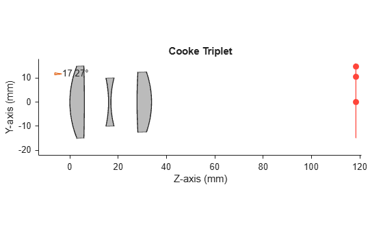

ans = 
  OpticalSystemViewer2D with properties:

            Title: ""
    OpticalSystem: [1×1 opticalSystem]
           Labels: "none"
      FieldPoints: "on"
             Rays: [0×0 optics.ui.Rays2D]
           Parent: [1×1 Figure]

  Show all properties

Specify the design wavelengths as the standard F (486.1 nm), d (587.6 nm), and C (656.3 nm) Fraunhofer lines spanning the visible spectrum. Define three field points, at 0, 5, and 7 degrees either in the horizontal or vertical direction, to capture different aberration sensitivities across the field. Focus the optical system at the mid-field point to balance on-axis and full-field performance.

opsys.Wavelengths = [486.1 587.6 656.3];
opsys.FieldPoints = fieldPoint(Angles=[0 0;0 5;7 0]);
focus(opsys,FieldPoint=opsys.FieldPoints(2),Wavelengths=opsys.Wavelengths);

Define Merit Function and Compensator

Define an optical merit function that evaluates the root mean square (RMS) spot size, which measures how tightly traced rays converge at the image plane. The merit function evaluates the spot size across all field points and wavelengths and returns a composite score. By default, the addSpot function uses all field points and wavelengths defined in the optical system to evaluate the spot size.

meritFcn = opticalMeritFunction;
meritFcn = addSpot(meritFcn)

meritFcn = 
  opticalMeritFunction with properties:

         Metrics: [1×1 optics.metric.SpotRMS]
         Weights: 1
    MetricsTable: [1×4 table]

Define a compensator that models the back-focus adjustment available during assembly. Image planes typically have a mechanical adjustment knob that enables you to shift the position of the detector along the optical axis. Because the Cooke triplet optical system has an image plane as its last component, you can add a compensator that moves the image plane within +/-0.2 mm along the Z-axis, which is the optical axis. During each sensitivity evaluation, the compensator moves the image plane within the permitted +/-0.2 mm range to the position that minimizes the merit function, so that reported contributions reflect the best achievable performance after focus adjustment. The found tolerances depend on this compensator range. A larger range allows looser tolerances, while a fixed-focus system requires significantly tighter tolerances.

numComponents = numel(opsys.Components);
compSet = opticalOptimizationSet;
compSet = addComponentPositionTuning(compSet,PositionZ=[-0.2 0.2],TargetIndex=numComponents);

Define Initial Tolerances

Define initial tolerances based on fabrication experience and manufacturer specifications. The initial tolerances represent the starting point for the iterative tolerancing process. The primary performance drivers for a Cooke triplet are the surface radius, the component thickness, the air gap, and the material properties such as refractive index and Abbe number.

Define tolerances for the surface radius by adding surface radius tolerances for all the curved surfaces, with a range of +/-0.1 mm, which is a typical test plate fit tolerance.

tolSet = opticalToleranceSet;
tolSet = addSurfaceRadiusTolerance(tolSet,[-0.1 0.1]);

Define tolerances for the component thickness by adding surface position tolerances for the terminating surfaces of each lens, with a range of +/-0.05 mm.

tolSet = addSurfacePositionTolerance(tolSet,PositionZ=[-0.05 0.05],TargetIndex=[2 4 6]);

Define tolerances for the air gap by adding component position tolerances for each lens, with a range of +/-0.08 mm.

numLensElements = numComponents-1;
tolSet = addComponentPositionTolerance(tolSet,PositionZ=[-0.08 0.08],TargetIndex=1:numLensElements);

Material tolerances account for melt-to-melt variation in glass properties. Refractive index (Nd) varies by approximately +/-0.0005 between melts of the same glass type for standard-grade glass, and Abbe number (Vd) varies by approximately +/-0.5. These values are representative starting points and actual tolerances depend on the glass type and supplier grade selected for production. Define tolerances for the material of components by adding tolerances for the refractive index (Nd) and Abbe number (Vd) of the component materials.

tolSet = addComponentMaterialTolerance(tolSet,Nd=[-0.0005 0.0005]);
tolSet = addComponentMaterialTolerance(tolSet,Vd=[-0.5 0.5]);

Run Forward Sensitivity Analysis

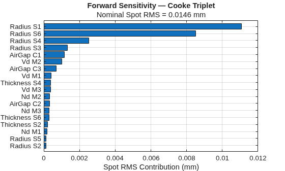
Run sensitivity analysis to identify the worst offenders, that is, the parameters that have the largest negative impact on the performance of the optical system when you perturb them to their current tolerance bounds. To run the sensitivity analysis, use the opticalSensitivity object function of the opticalSystem object. The opticalSensitivity function perturbs each tolerance parameter once to its upper bound and once to its lower bound, optimizes the compensator, and records the worst-case spot size degradation.

sensResult = opticalSensitivity(opsys,meritFcn,tolSet,Compensator=compSet,UseParallel=true);
nominalVal = sensResult.NominalMeritValue;
tbl = sensResult.ResultTable;
numTol = height(tbl);
paramNames = tbl.TargetProperty;
targetIndices = tbl.TargetIndex;
paramTypes = tbl.TargetPropertyType;

Extract the forward contributions of each parameter, using the extractContributions function, which is defined at the end of this example. The forward contribution of each parameter measures its worst-case impact on the merit function when the parameter value is perturbed to its tolerance bounds. For parameter k with tolerance range [-t, +t], the opticalSensitivity function evaluates the optical system at both bounds while the compensator is optimized, producing two perturbed spot sizes. The contribution of each parameter is

contribution(k) = max(abs(spot_plus(k)-spot_nominal),abs(spot_minus(k)-spot_nominal))

where spot_nominal is the unperturbed root mean square (RMS) spot size, spot_plus(k) is the RMS spot size when parameter k is perturbed to its upper bound, and spot_minus(k) is the RMS spot size when parameter k is perturbed to its lower bound. The sensitivity analysis considers the larger of the two deviations because the system might be asymmetrically sensitive to positive and negative perturbations.

Create display labels for visualization, using the makeLabels supporting function, which is defined at the end of this example.

fwdContrib = extractContributions(tbl,nominalVal);
labels = makeLabels(paramNames,targetIndices,paramTypes);

Visualize the forward sensitivity results as a horizontal bar chart sorted by contribution magnitude. Parameters at the top of the chart are the most sensitive and need the tightest tolerances.

[sortedFwdContrib,sortIdx] = sort(fwdContrib,"ascend");
figure(Name="Forward Sensitivity")
barh(categorical(labels(sortIdx),labels(sortIdx)),sortedFwdContrib)
xlabel("Spot RMS Contribution (mm)")
title("Forward Sensitivity — Cooke Triplet")
subtitle(compose("Nominal Spot RMS = %.4f mm",nominalVal))
grid on

Run Inverse Sensitivity Analysis

Forward sensitivity analysis shows which parameters are most sensitive, but it does not indicate what tolerance value should appear on the manufacturing drawing. Inverse sensitivity analysis answers this reverse question: Given a performance specification, what is the maximum allowable tolerance for each parameter?

Specification and Budget

Set the RMS spot size specification to 0.016 mm. This is a practical manufacturing target that balances image quality against fabrication cost. A specification too close to the nominal value leaves almost no RSS budget, forcing impractically tight tolerances. A specification too far from the nominal value makes every parameter insensitive, providing no useful guidance. The total tolerance budget is the difference between the specification and the nominal performance using the RSS relationship.

spotSpec = 0.016; % mm RMS
totalBudget = sqrt(spotSpec^2-nominalVal^2);

Manufacturing errors across different parameters (radius of surface 1, thickness of surface 4, index of material 2, and so on) are statistically independent. When independent errors combine, the total is not their arithmetic sum but their RSS. For example, if three parameters each contribute an error of 0.002 mm, the combined total is not 0.002 + 0.002 + 0.002 = 0.006 mm but sqrt(0.002^2 + 0.002^2 + 0.002^2) = 0.0035 mm. The RSS total is smaller than the linear sum because it is unlikely that every parameter simultaneously reaches its worst-case perturbation bound.

Bisection Search with Iterative Budget Reallocation

The simplest approach is to divide the total budget equally among all parameters.

perParamBudget = totalBudget/sqrt(N)

However, equal allocation is wasteful because insensitive parameters hit their practical manufacturing ceilings without using their full budget shares, leaving the constrained parameters with tighter tolerances than necessary.

To fully utilize the available budget, apply iterative reallocation by using the getMaxSearchRange and allocateBudgetIteratively supporting functions, which are defined at the end of this example. Follow these steps:

1. Start with equal allocation across all parameters.

2. Run bisection search to find the maximum tolerance for each parameter within its budget.

3. A parameter that hits their manufacturing ceiling is insensitive, because it uses less budget than allocated. Compute the actual contribution of each insensitive parameter at its ceiling tolerance.

4. Subtract the insensitive contributions from the total budget, and redistribute the remaining budget equally among only the constrained parameters.

5. Rerun bisection search for the constrained parameters with their new, larger budget.

6. Repeat steps 1 through 5 until the allocation is stable. Typically, 2–3 iterations suffice.

maxSearchRange = getMaxSearchRange(paramNames);
[foundTol,perParamBudgets] = allocateBudgetIteratively(opsys,meritFcn, ...
    compSet,nominalVal,totalBudget,paramNames,paramTypes, ...
    targetIndices,maxSearchRange);

The bisection searches within a range from near-zero up to a manufacturing ceiling for each parameter. The ceiling is the loosest tolerance. These are the loose tolerance defined for each parameter.

• +/-0.2 mm for geometric parameters (radius, thickness, air gap)

• +/-0.001 for refractive index (Nd, standard catalog glass melt tolerance)

• +/-1 for Abbe number (Vd)

The manufacturing drawing specifies the found tolerance from the bisection search. For example, if a surface has a nominal radius of 50 mm and bisection finds a tolerance of 0.059 mm, the drawing specifies "R = 50 +/-0.059 mm", which means that the fabricated radius must fall between 49.941 mm and 50.059 mm. A parameter whose found tolerance equals its ceiling is insensitive, and a parameter whose found tolerance is below its ceiling is constrained and is a cost driver.

Tolerance Summary Table

The summary table presents the inverse sensitivity results. Each parameter is classified as either "Constrained" or "At limit".

• "Constrained" — The found tolerance is below the search ceiling. This parameter actively consumes RSS budget and is a cost driver. Tightening or loosening it directly affects the predicted performance.

• "At limit" — The found tolerance has reached the search ceiling (0.2 mm for geometric, 0.001 for Nd, 1 for Vd). This parameter is insensitive at this specification. Even the loosest practical manufacturing variation does not consume significant budget. These parameters can be set to standard shop practice without affecting yield. Seeing many parameters "At limit" is normal and expected. It means that only a handful of parameters drive performance, which is typical for well-optimized optical designs.

Visualize the tolerance summary as a table.

getStatus = strings(numTol,1);
for tolIdx = 1:numTol
    if foundTol(tolIdx)>=maxSearchRange(tolIdx)-1e-6
        getStatus(tolIdx) = "At limit";
    else
        getStatus(tolIdx) = "Constrained";
    end
end

summaryTable = table(labels,fwdContrib,foundTol,getStatus, ...
    VariableNames=["Parameter","FwdContribution_mm", ...
    "FoundTolerance_mm","Status"])

summaryTable = 18×4 table
      Parameter       FwdContribution_mm    FoundTolerance_mm       Status    
    ______________    __________________    _________________    _____________

    "Radius S6"            0.0085134             0.059376        "Constrained"
    "Radius S1"             0.011067             0.065626        "Constrained"
    "Radius S4"             0.002534             0.084376        "Constrained"
    "Radius S3"            0.0013272              0.10938        "Constrained"
    "Vd M2"                0.0010105              0.82813        "Constrained"
    "AirGap C1"            0.0011547             0.084376        "Constrained"
    "AirGap C3"           0.00069765                  0.2        "At limit"   
    "Vd M1"                0.0004153                    1        "At limit"   
    "Nd M2"                0.0003336           0.00085952        "Constrained"
    "Vd M3"               0.00038695                    1        "At limit"   
    "Thickness S4"        0.00039774                  0.2        "At limit"   
    "Nd M3"               0.00030144                0.001        "At limit"   
    "Thickness S6"         0.0003003                  0.2        "At limit"   
    "AirGap C2"           0.00033059              0.11563        "Constrained"
    "Thickness S2"         0.0002259              0.18438        "Constrained"
    "Nd M1"               0.00017575           0.00098439        "Constrained"
      ⋮

Found Tolerances

Obtain the initial tolerances by using the getInitialTolerance supporting function, which is defined at the end of this example.

initialTol = zeros(numTol,1);
for tolIdx = 1:numTol
    initialTol(tolIdx) = getInitialTolerance(paramNames(tolIdx),paramTypes(tolIdx));
end

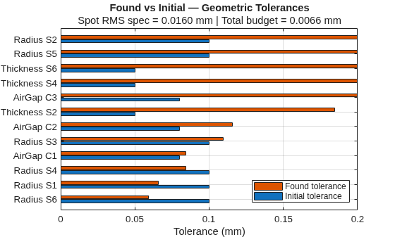
Visualize the found tolerances side by side with the initial tolerances. This comparison shows which parameters are tightened (the found tolerance is less than the initial tolerance), which are unchanged, and which are relaxed (the found tolerance is greater than the initial tolerance).

Separate the geometric and material tolerances.

isGeometric = ~(paramNames== "Nd"|paramNames=="Vd");

Visualize geometric parameters, such as radius, thickness, and air gap, in mm in one plot.

geoIdx = find(isGeometric);
[~,geoSort] = sort(foundTol(geoIdx),"ascend");
geoIdx = geoIdx(geoSort);
figure(Name="Found vs Initial — Geometric Tolerances")
barh(categorical(labels(geoIdx),labels(geoIdx)), ...
    [initialTol(geoIdx) foundTol(geoIdx)]);
xlabel("Tolerance (mm)")
title("Found vs Initial — Geometric Tolerances")
subtitle(compose("Spot RMS spec = %.4f mm | Total budget = %.4f mm", ...
    spotSpec, totalBudget))
legend("Initial tolerance","Found tolerance",Location="southeast")
grid on

Visualize the material parameters Nd and Vd, which have different units, in a separate plot.

matIdx = find(~isGeometric);
[~, matSort] = sort(foundTol(matIdx),"ascend");
matIdx = matIdx(matSort);
figure(Name="Found vs Initial — Material Tolerances")
barh(categorical(labels(matIdx),labels(matIdx)), ...
    [initialTol(matIdx) foundTol(matIdx)]);
xlabel("Tolerance (Nd or Vd units)")
title("Found vs Initial — Material Tolerances")
legend("Initial tolerance","Found tolerance",Location="southeast")
grid on

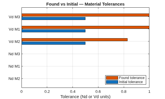
These plots compare the found tolerances from the inverse sensitivity analysis against the initial tolerances. Parameters where the found tolerance is smaller than the initial tolerance must be tightened beyond the starting value to meet the specification, because these parameters are cost drivers. Parameters where the found tolerance is larger than the initial tolerance were over-toleranced initially and can be relaxed.

Per-Parameter Contribution vs Budget

Compute the contribution of each parameter at its found tolerance, using the evaluateAllParams supporting function, which is defined at the end of this example.

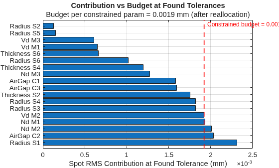
Plot the budget of each parameter as a horizontal bar chart against the worst-case contribution of each parameter at its found tolerance. Constrained parameters have bars that reach the budget line as the bisection process tightens their tolerance until their contribution matches the allocated budget. Insensitive parameters have shorter bars because they hit their manufacturing ceiling before their contribution can grow large enough to reach the budget line.

Some constrained parameters can slightly exceed the budget line because the bisection process uses a finite number of iterations and converges within a small tolerance rather than to an exact value. These small overshoots do not violate the specification, because the pass/fail criterion is the total RSS of all contributions, not on any individual parameter staying below the line.

foundContrib = evaluateAllParams(opsys,meritFcn,compSet,nominalVal, ...
    paramNames,paramTypes,targetIndices,foundTol,UseParallel=true);

[~,sortIdx] = sort(foundContrib,"descend");

% Use the budget allocated to constrained parameters for the reference line
constrainedBudget = max(perParamBudgets);

figure(Name="Per-Parameter Contribution vs Budget")
barh(categorical(labels(sortIdx), labels(sortIdx)), foundContrib(sortIdx))
hold on
xline(constrainedBudget,"r--",compose("Constrained budget = %.4f mm",constrainedBudget), ...
    LineWidth=1.5,FontSize=9,LabelOrientation="horizontal")
hold off
xlabel("Spot RMS Contribution at Found Tolerance (mm)")
title("Contribution vs Budget at Found Tolerances")
subtitle(compose("Budget per constrained param = %.4f mm (after reallocation)", ...
    constrainedBudget))
grid on

RSS Waterfall

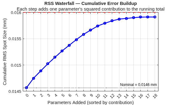
To visualize how the contribution of each parameter accumulates toward the total RSS error, create a waterfall plot. The waterfall starts from the nominal spot size and adds the squared contribution of each parameter in order of decreasing magnitude. The final point shows the predicted total spot size relative to the specification.

The waterfall plot shows which parameters consume the most budget and how much budget remains. The steep initial steps correspond to the most sensitive parameters, which consume the most budget. The curve flattens as insensitive parameters add negligible contribution. If the final point reaches or touches the red specification line, the design uses the full budget. A gap between the final point and the specification line indicates unused budget, typically from insensitive parameters that hit their ceiling before exhausting their share of the budget.

sortedFoundContrib = sort(foundContrib,"descend");
cumulativeRSS = cumsum([nominalVal^2; sortedFoundContrib.^2]);
cumulativeSpot = sqrt(cumulativeRSS);

figure(Name="RSS Waterfall — Cumulative Error Buildup");
plot(0:numTol, cumulativeSpot,"b-o",LineWidth=2,MarkerSize=5);
hold on
yline(spotSpec,"r--",compose("Spec = %.4f mm",spotSpec), ...
    LineWidth=1.5,FontSize=10)
yline(nominalVal,"k:",compose("Nominal = %.4f mm",nominalVal), ...
    LineWidth=1,FontSize=9);
hold off
xlabel("Parameters Added (sorted by contribution)")
ylabel("Cumulative RMS Spot Size (mm)")
title("RSS Waterfall — Cumulative Error Buildup")
subtitle("Each step adds one parameter's squared contribution to the running total")
xticks(0:numTol)
xlim([-0.5 numTol+0.5])
grid on

Verify Found Tolerances

Rebuild the tolerance set by using the buildToleranceSet supporting function, which is defined at the end of this example. Verify that the found tolerances satisfy the specification by rerunning the forward sensitivity analysis at the found tolerance values. reevaluating the contribution of each parameter independently. If the bisection converged correctly, the RSS-predicted total spot size is at or below the specification.

tolSetVerify = buildToleranceSet(paramNames,paramTypes,targetIndices,foundTol);
verifResult = opticalSensitivity(opsys,meritFcn,tolSetVerify,Compensator=compSet,UseParallel=true);
verifContrib = extractContributions(verifResult.ResultTable,nominalVal);
verifRSS = sqrt(sum(verifContrib.^2));
predictedTotal = sqrt(nominalVal^2+verifRSS^2);

if predictedTotal<=spotSpec
    passStr = "PASS";
else
    passStr = "FAIL";
end

disp("  RSS-predicted spot size: " + compose("%.4f",predictedTotal) + " mm");

  RSS-predicted spot size: 0.0159 mm

disp("  Specification: " + compose("%.4f",spotSpec) + " mm");

  Specification: 0.0160 mm

disp("  Result: " + passStr);

  Result: PASS

The resulting tolerance table is ready for manufacturing review. However, the RSS verification is a conservative analytical estimate. It evaluates each parameter at its worst-case bound, then combines contributions via root-sum-square. In practice, manufacturing errors are random and can partially cancel one another out, so the real-world performance is almost always better than the RSS prediction. To evaluate how these tolerances perform under realistic random manufacturing errors, and to iteratively improve yield through targeted tightening and compensator widening, see the companion example Improve Manufacturing Yield Using Monte Carlo Analysis.

Supporting Functions

extractContributions

This function computes the worst-case spot size contribution for each parameter. For each row, the function takes the maximum absolute deviation from the nominal value across both perturbation bounds.

function contrib = extractContributions(T,nominalVal)
    numTol = height(T);
    contrib = zeros(numTol,1);
    for idx = 1:numTol
        scores = T.MetricScore{idx};
        contrib(idx) = max(abs(scores{1}-nominalVal), ...
            abs(scores{2}-nominalVal));
    end
end

makeLabels

This function creates display labels for each tolerance parameter by combining the tolerance type with the target index.

function labels = makeLabels(paramNames,targetIndices,paramTypes)
    numTol = numel(paramNames);
    labels = strings(numTol,1);
    for idx = 1:numTol
        if paramNames(idx)=="Radius"
            labels(idx) = "Radius S" + string(targetIndices(idx));
        elseif contains(paramTypes(idx),"SurfacePosition")
            labels(idx) = "Thickness S" + string(targetIndices(idx));
        elseif contains(paramTypes(idx),"ComponentPosition")
            labels(idx) = "AirGap C" + string(targetIndices(idx));
        elseif paramNames(idx)=="Nd"
            labels(idx) = "Nd M" + string(targetIndices(idx));
        elseif paramNames(idx)=="Vd"
            labels(idx) = "Vd M" + string(targetIndices(idx));
        end
    end
end

getMaxSearchRange

This function returns a per-parameter search ceiling vector. The elements of the vector represent the loosest tolerances that a fabrication shop might realistically hold: +/-0.2 mm for geometric parameters, +/-0.001 for Nd (lowest-grade glass melt tolerance), and +/-1 for Vd. Any found tolerance at or near these values means that the parameter is insensitive and can be set to the standard shop practice value.

function maxRange = getMaxSearchRange(paramNames)
    numTol = numel(paramNames);
    maxRange = zeros(numTol,1);
    for idx = 1:numTol
        if paramNames(idx)=="Nd"
            maxRange(idx) = 0.001;
        elseif paramNames(idx)=="Vd"
            maxRange(idx) = 1;
        else
            maxRange(idx) = 0.2;
        end
    end
end

allocateBudgetIteratively

This function iteratively allocates the total RSS budget across parameters. In each iteration, the function evaluates the actual contributions of the insensitive parameters, then redistributes the remaining budget equally among only the constrained parameters. These steps repeat until no new parameters become insensitive, indicating that the budget is fully utilized. This function uses the runBisection and evalSelectedParams supporting functions, which are defined later in this section.

function [foundTol,perParamBudgets] = allocateBudgetIteratively(opsys, ...
    meritFcn,compSet,nominalVal,totalBudget,paramNames,paramTypes, ...
    targetIndices,maxSearchRange,options)

    arguments
        opsys
        meritFcn
        compSet
        nominalVal
        totalBudget
        paramNames
        paramTypes
        targetIndices
        maxSearchRange
        options.UseParallel {matlab.internal.parallel.validateUseParallelOption} = "off"
    end
    
    numTol = numel(paramNames);
    maxReallocationIter = 5;
    
    % Start with equal allocation
    perParamBudgets = repmat(totalBudget/sqrt(numTol),numTol,1);
    isInsensitive = false(numTol,1);
    insensitiveContrib = zeros(numTol,1);
    
    pool = matlab.internal.parallel.resolveUseParallel(options.UseParallel);
    
    for reallocationIter = 1:maxReallocationIter
        % Run bisection with current budget allocation
        foundTol = runBisection(opsys,meritFcn,compSet,nominalVal, ...
            paramNames,paramTypes,targetIndices,perParamBudgets, ...
            maxSearchRange,pool);
    
        % Identify insensitive parameters (hit the ceiling)
        newInsensitive = (foundTol>=maxSearchRange-1e-6);
    
        % Check convergence: no new insensitive parameters found
        if isequal(newInsensitive,isInsensitive)
            break;
        end
        isInsensitive = newInsensitive;
    
        % Measure actual contributions of insensitive parameters
        insensIdx = find(isInsensitive);
        insensContribLocal = evalSelectedParams(opsys,meritFcn,compSet, ...
            nominalVal,paramNames,paramTypes,targetIndices,foundTol, ...
            insensIdx,pool);
        insensitiveContrib(insensIdx) = insensContribLocal;
    
        % Compute remaining budget after insensitive contributions are subtracted
        usedBudgetSq = sum(insensitiveContrib(isInsensitive).^2);
        remainingBudgetSq = totalBudget^2-usedBudgetSq;
    
        if remainingBudgetSq<=0
            break;
        end
    
        % Redistribute remaining budget equally among constrained parameters
        numConstrained = sum(~isInsensitive);
        if numConstrained == 0
            break;
        end
        constrainedBudget = sqrt(remainingBudgetSq)/sqrt(numConstrained);
    
        % Update per-parameter budgets
        perParamBudgets(isInsensitive) = insensitiveContrib(isInsensitive);
        perParamBudgets(~isInsensitive) = constrainedBudget;
    end
end

runBisection

This function performs an independent bisection search for each parameter. If a parallel pool is available, the function searches all parameters concurrently on pool workers, using parallel.pool.Constant to broadcast the handle objects. Otherwise, the search runs sequentially. This function uses the evalSingleParam supporting function, which is defined later in this section.

function foundTol = runBisection(opsys,meritFcn,compSet,nominalVal, ...
    paramNames,paramTypes,targetIndices,perParamBudgets,maxSearchRange,pool)

    numTol = numel(paramNames);
    foundTol = zeros(numTol,1);
    maxIter = 5;
    
    if ~isempty(pool)
        % Parallel: broadcast handle objects to workers once
        opsysConst = parallel.pool.Constant(opsys);
        compSetConst = parallel.pool.Constant(compSet);
    
        parfor idx = 1:numTol
            prop = paramNames(idx);
            ptype = paramTypes(idx);
            tidx = targetIndices(idx);
    
            lo = 1e-6;
            hi = maxSearchRange(idx);
            budget_k = perParamBudgets(idx);
    
            hiVal = evalSingleParam(opsysConst.Value, meritFcn, ...
                compSetConst.Value, nominalVal, prop, ptype, tidx, hi);
    
            if hiVal <= budget_k
                foundTol(idx) = hi;
            else
                for iter = 1:maxIter
                    mid = (lo + hi) / 2;
                    midVal = evalSingleParam(opsysConst.Value,meritFcn, ...
                        compSetConst.Value,nominalVal,prop,ptype,tidx,mid);
                    if midVal > budget_k
                        hi = mid;
                    else
                        lo = mid;
                    end
                    if (hi-lo)/max(mid,1e-10)<0.03
                        break;
                    end
                end
                foundTol(idx) = (lo+hi)/2;
            end
        end
    
        delete(opsysConst);
        delete(compSetConst);
    else
        % Serial
        for idx = 1:numTol
            prop = paramNames(idx);
            ptype = paramTypes(idx);
            tidx = targetIndices(idx);
    
            lo = 1e-6;
            hi = maxSearchRange(idx);
            budget_k = perParamBudgets(idx);
    
            hiVal = evalSingleParam(opsys,meritFcn,compSet,nominalVal, ...
                prop,ptype,tidx,hi);
    
            if hiVal <= budget_k
                foundTol(idx) = hi;
            else
                for iter = 1:maxIter
                    mid = (lo+hi)/2;
                    midVal = evalSingleParam(opsys,meritFcn,compSet, ...
                        nominalVal,prop,ptype,tidx,mid);
                    if midVal>budget_k
                        hi = mid;
                    else
                        lo = mid;
                    end
                    if (hi-lo)/max(mid,1e-10)<0.03
                        break;
                    end
                end
                foundTol(idx) = (lo+hi)/2;
            end
        end
    end
end

evalSelectedParams

This function measures the contributions of insensitive parameters during budget reallocation by evaluating these parameters (specified by index) at their found tolerances.

function contrib = evalSelectedParams(opsys,meritFcn,compSet,nominalVal, ...
    paramNames,paramTypes,targetIndices,tolValues,selectedIdx,pool)

    numSelected = numel(selectedIdx);
    contrib = zeros(numSelected,1);
    
    if ~isempty(pool)
        opsysConst = parallel.pool.Constant(opsys);
        compSetConst = parallel.pool.Constant(compSet);
        parfor idx = 1:numSelected
            selIdx = selectedIdx(idx);
            contrib(idx) = evalSingleParam(opsysConst.Value,meritFcn, ...
                compSetConst.Value,nominalVal, ...
                paramNames(selIdx),paramTypes(selIdx),targetIndices(selIdx),tolValues(selIdx));
        end
        delete(opsysConst);
        delete(compSetConst);
    else
        for idx = 1:numSelected
            selIdx = selectedIdx(idx);
            contrib(idx) = evalSingleParam(opsys,meritFcn,compSet,nominalVal, ...
                paramNames(selIdx),paramTypes(selIdx),targetIndices(selIdx),tolValues(selIdx));
        end
    end
end

evalSingleParam

This function evaluates the spot size contribution for a single parameter at a given tolerance value. Parallelism is disabled within this function because it is called from inside parfor workers . The outer parameter loop provides the parallelism instead.

function val = evalSingleParam(opsys,meritFcn,compSet,nomVal, ...
    prop,ptype,tidx,tolVal)

    tolSet = buildToleranceSet(prop,ptype,tidx,tolVal);
    
    result = opticalSensitivity(opsys,meritFcn,tolSet, ...
        Compensator=compSet,UseParallel=false);
    Tres = result.ResultTable;
    scores = Tres.MetricScore{1};
    val = max(abs(scores{1}-nomVal),abs(scores{2}-nomVal));
end

evaluateAllParams

This function evaluates all parameters at their found tolerances. If a parallel pool is available, the function runs the evaluations concurrently, using parallel.pool.Constant to broadcast handle objects.

function contrib = evaluateAllParams(opsys,meritFcn,compSet,nominalVal, ...
    paramNames,paramTypes,targetIndices,tolValues,options)

    arguments
        opsys
        meritFcn
        compSet
        nominalVal
        paramNames
        paramTypes
        targetIndices
        tolValues
        options.UseParallel {matlab.internal.parallel.validateUseParallelOption} = "off"
    end
    
    numTol = numel(paramNames);
    contrib = zeros(numTol,1);
    pool = matlab.internal.parallel.resolveUseParallel(options.UseParallel);
    
    if ~isempty(pool)
        opsysConst = parallel.pool.Constant(opsys);
        compSetConst = parallel.pool.Constant(compSet);
        parfor idx = 1:numTol
            contrib(idx) = evalSingleParam(opsysConst.Value,meritFcn, ...
                compSetConst.Value,nominalVal, ...
                paramNames(idx),paramTypes(idx),targetIndices(idx),tolValues(idx));
        end
        delete(opsysConst);
        delete(compSetConst);
    else
        for idx = 1:numTol
            contrib(idx) = evalSingleParam(opsys,meritFcn,compSet,nominalVal, ...
                paramNames(idx),paramTypes(idx),targetIndices(idx),tolValues(idx));
        end
    end
end

getInitialTolerance

This function returns the initial tolerance half-range for a parameter based on its type.

function ft = getInitialTolerance(paramName,paramType)
    if paramName=="Radius"
        ft = 0.1;
    elseif contains(paramType,"SurfacePosition")
        ft = 0.05;
    elseif contains(paramType,"ComponentPosition")
        ft = 0.08;
    elseif paramName=="Nd"
        ft = 0.0005;
    elseif paramName=="Vd"
        ft = 0.5;
    else
        ft = 0;
    end
end

buildToleranceSet

This function constructs an opticalToleranceSet from per-parameter tolerance values, dispatching to the correct API function for each parameter type.

function tolSet = buildToleranceSet(paramNames,paramTypes,targetIndices,tolValues)
    tolSet = opticalToleranceSet;
    for numParams = 1:numel(paramNames)
        ft = tolValues(numParams);
        if paramNames(numParams)=="Radius"
            tolSet = addSurfaceRadiusTolerance(tolSet,[-ft, ft], ...
                TargetIndex=targetIndices(numParams));
        elseif contains(paramTypes(numParams),"SurfacePosition")
            tolSet = addSurfacePositionTolerance(tolSet,PositionZ=[-ft, ft], ...
                TargetIndex=targetIndices(numParams));
        elseif contains(paramTypes(numParams),"ComponentPosition")
            tolSet = addComponentPositionTolerance(tolSet,PositionZ=[-ft, ft], ...
                TargetIndex=targetIndices(numParams));
        elseif paramNames(numParams)=="Nd"
            tolSet = addComponentMaterialTolerance(tolSet,Nd=[-ft, ft], ...
                TargetIndex=targetIndices(numParams));
        elseif paramNames(numParams)=="Vd"
            tolSet = addComponentMaterialTolerance(tolSet,Vd=[-ft, ft], ...
                TargetIndex=targetIndices(numParams));
        end
    end
end