Differential Equations
This example shows how to use MATLAB® to formulate and solve several different types of differential equations. MATLAB offers several numerical algorithms to solve a wide variety of differential equations:
Initial value problems
Boundary value problems
Delay differential equations
Partial differential equations
Initial Value Problem
vanderpoldemo is a function that defines the van der Pol equation
type vanderpoldemofunction dydt = vanderpoldemo(t,y,Mu) %VANDERPOLDEMO Defines the van der Pol equation for ODEDEMO. % Copyright 1984-2014 The MathWorks, Inc. dydt = [y(2); Mu*(1-y(1)^2)*y(2)-y(1)];
The equation is written as a system of two first-order ordinary differential equations (ODEs). These equations are evaluated for different values of the parameter . For faster integration, you should choose an appropriate solver based on the value of .
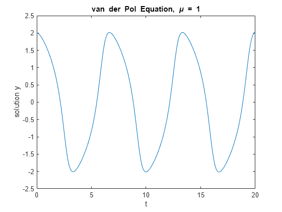
For , any of the MATLAB ODE solvers can solve the van der Pol equation efficiently. The ode45 solver is one such example. The equation is solved in the domain with the initial conditions and .
tspan = [0 20];
y0 = [2; 0];
Mu = 1;
ode = @(t,y) vanderpoldemo(t,y,Mu);
[t,y] = ode45(ode, tspan, y0);

% Plot solution
plot(t,y(:,1))
xlabel('t')
ylabel('solution y')
title('van der Pol Equation, \mu = 1')
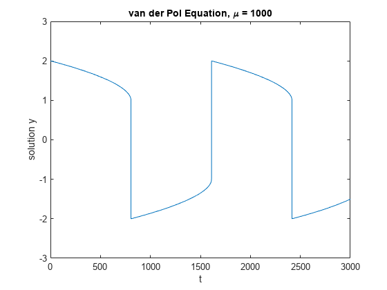
For larger magnitudes of , the problem becomes stiff. This label is for problems that resist attempts to be evaluated with ordinary techniques. Instead, special numerical methods are needed for fast integration. The ode15s, ode23s, ode23t, and ode23tb functions can solve stiff problems efficiently.
This solution to the van der Pol equation for uses ode15s with the same initial conditions. You need to stretch out the time span drastically to to be able to see the periodic movement of the solution.
tspan = [0, 3000];
y0 = [2; 0];
Mu = 1000;
ode = @(t,y) vanderpoldemo(t,y,Mu);
[t,y] = ode15s(ode, tspan, y0);

plot(t,y(:,1))
title('van der Pol Equation, \mu = 1000')
axis([0 3000 -3 3])
xlabel('t')
ylabel('solution y')
Boundary Value Problems
bvp4c and bvp5c solve boundary value problems for ordinary differential equations.
The example function twoode has a differential equation written as a system of two first-order ODEs. The differential equation is
type twoodefunction dydx = twoode(x,y) %TWOODE Evaluate the differential equations for TWOBVP. % % See also TWOBC, TWOBVP. % Lawrence F. Shampine and Jacek Kierzenka % Copyright 1984-2014 The MathWorks, Inc. dydx = [ y(2); -abs(y(1)) ];
The function twobc has the boundary conditions for the problem: and .
type twobcfunction res = twobc(ya,yb) %TWOBC Evaluate the residual in the boundary conditions for TWOBVP. % % See also TWOODE, TWOBVP. % Lawrence F. Shampine and Jacek Kierzenka % Copyright 1984-2014 The MathWorks, Inc. res = [ ya(1); yb(1) + 2 ];
Prior to calling bvp4c, you have to provide a guess for the solution you want represented at a mesh. The solver then adapts the mesh as it refines the solution.
The bvpinit function assembles the initial guess in a form you can pass to the solver bvp4c. For a mesh of [0 1 2 3 4] and constant guesses of and , the call to bvpinit is:
solinit = bvpinit([0 1 2 3 4],[1; 0]);
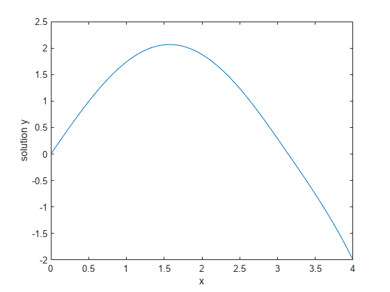
With this initial guess, you can solve the problem with bvp4c. Evaluate the solution returned by bvp4c at some points using deval, and then plot the resulting values.
sol = bvp4c(@twoode, @twobc, solinit);

xint = linspace(0, 4, 50);
yint = deval(sol, xint);
plot(xint, yint(1,:));
xlabel('x')
ylabel('solution y')
hold on
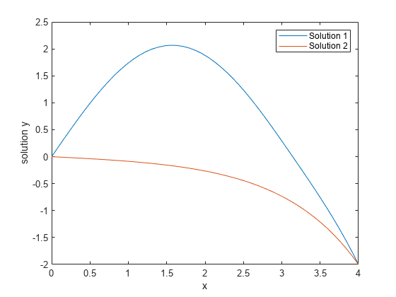
This particular boundary value problem has exactly two solutions. You can obtain the other solution by changing the initial guesses to and .
solinit = bvpinit([0 1 2 3 4],[-1; 0]);
sol = bvp4c(@twoode,@twobc,solinit);

xint = linspace(0,4,50);
yint = deval(sol,xint);
plot(xint,yint(1,:));
legend('Solution 1','Solution 2')
hold off
Delay Differential Equations
dde23, ddesd, and ddensd solve delay differential equations with various delays. The examples ddex1, ddex2, ddex3, ddex4, and ddex5 form a mini tutorial on using these solvers.
The ddex1 example shows how to solve the system of differential equations
You can represent these equations with the anonymous function
ddex1fun = @(t,y,Z) [Z(1,1); Z(1,1)+Z(2,2); y(2)];
The history of the problem (for ) is constant:
You can represent the history as a vector of ones.
ddex1hist = ones(3,1);
A two-element vector represents the delays in the system of equations.
lags = [1 0.2];
Pass the function, delays, solution history, and interval of integration to the solver as inputs. The solver produces a continuous solution over the whole interval of integration that is suitable for plotting.
sol = dde23(ddex1fun, lags, ddex1hist, [0 5]);

plot(sol.x,sol.y);
title({'An example of Wille and Baker', 'DDE with Constant Delays'});
xlabel('time t');
ylabel('solution y');
legend('y_1','y_2','y_3','Location','NorthWest');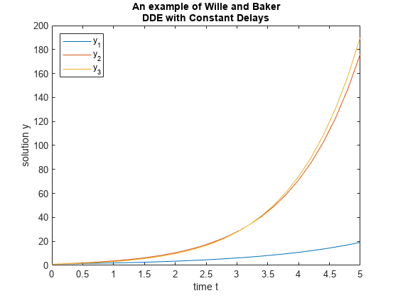
Partial Differential Equations
pdepe solves partial differential equations in one space variable and time. The examples pdex1, pdex2, pdex3, pdex4, and pdex5 form a mini tutorial on using pdepe.
This example problem uses the functions pdex1pde, pdex1ic, and pdex1bc.
pdex1pde defines the differential equation
type pdex1pdefunction [c,f,s] = pdex1pde(x,t,u,DuDx) %PDEX1PDE Evaluate the differential equations components for the PDEX1 problem. % % See also PDEPE, PDEX1. % Lawrence F. Shampine and Jacek Kierzenka % Copyright 1984-2014 The MathWorks, Inc. c = pi^2; f = DuDx; s = 0;
pdex1ic sets up the initial condition
type pdex1icfunction u0 = pdex1ic(x) %PDEX1IC Evaluate the initial conditions for the problem coded in PDEX1. % % See also PDEPE, PDEX1. % Lawrence F. Shampine and Jacek Kierzenka % Copyright 1984-2014 The MathWorks, Inc. u0 = sin(pi*x);
pdex1bc sets up the boundary conditions
type pdex1bcfunction [pl,ql,pr,qr] = pdex1bc(xl,ul,xr,ur,t) %PDEX1BC Evaluate the boundary conditions for the problem coded in PDEX1. % % See also PDEPE, PDEX1. % Lawrence F. Shampine and Jacek Kierzenka % Copyright 1984-2014 The MathWorks, Inc. pl = ul; ql = 0; pr = pi * exp(-t); qr = 1;
pdepe requires the spatial discretization x and a vector of times t (at which you want a snapshot of the solution). Solve the problem using a mesh of 20 nodes and request the solution at five values of t. Extract and plot the first component of the solution.
x = linspace(0,1,20);
t = [0 0.5 1 1.5 2];
sol = pdepe(0,@pdex1pde,@pdex1ic,@pdex1bc,x,t);

u1 = sol(:,:,1);

surf(x,t,u1);
xlabel('x');
ylabel('t');
zlabel('u');

See Also
Related Topics
You can also select a web site from the following list:
Americas
- América Latina (Español)
- Canada (English)
- United States (English)
Europe
- Belgium (English)
- Denmark (English)
- Deutschland (Deutsch)
- España (Español)
- Finland (English)
- France (Français)
- Ireland (English)
- Italia (Italiano)
- Luxembourg (English)
- Netherlands (English)
- Norway (English)
- Österreich (Deutsch)
- Portugal (English)
- Sweden (English)
- Switzerland
- United Kingdom (English)