Compare Point Clouds in Point Cloud Analyzer

R2026b

Since R2026b

This example shows how to compare two point clouds to detect changes using the Point Cloud Analyzer app.

Comparing point clouds captured at different times helps you perform change detection tasks such as urban monitoring and infrastructure analysis. This example uses urban development as a scenario. The same workflow applies to any application where you need to quantify geometric differences between point clouds.

In this example, you:

• Load two lidar point clouds of the same area captured at different times.

• Import the point clouds into the Point Cloud Analyzer app.

• Use the Compare feature to compute distances between the point clouds.

• Visualize differences as a distance heatmap.

• Interpret comparison metrics.

Download and Prepare Point Cloud Data

This example uses lidar data from the U.S. Geological Survey (USGS) 3D Elevation Program (3DEP) publicly available through the USGS Lidar Explorer. This platform provides recorded lidar data in LAZ format for locations across the United States.

To see real-world changes over time, download lidar survey data acquired in 2013 and 2023 near the University of Utah in Salt Lake City. The 2013 survey includes RGB color information, while the 2023 survey does not. This difference does not affect the geometric comparison. Comparing these surveys reveals 10 years of urban development, including new buildings, demolished structures, and renovated buildings.

Download the point cloud data from the USGS rockyweb server.

url2013 = "https://rockyweb.usgs.gov/vdelivery/Datasets/Staged/" + ...
    "Elevation/LPC/Projects/Wasatch_Fault_UT_LiDAR/UT_Wasatch_L4_2013/" + ...
    "LAZ/USGS_LPC_Wasatch_Fault_UT_LiDAR_12TVL2900012000.laz";
url2023 = "https://rockyweb.usgs.gov/vdelivery/Datasets/Staged/" + ...
    "Elevation/LPC/Projects/UT_2023SaltLakeCo_C24/UT_2023_SaltLakeCo_1_C24/" + ...
    "LAZ/USGS_LPC_UT_2023SaltLakeCo_C24_12TVL2912.laz";
outputFolder = fullfile(tempdir,"saltlake_comparison");
if ~exist(outputFolder,"dir")
    mkdir(outputFolder);
end
file2013 = fullfile(outputFolder,"SaltLake_2013.laz");
file2023 = fullfile(outputFolder,"SaltLake_2023.laz");
opts = weboptions(Timeout=180);
if ~isfile(file2013)
    disp("Downloading SaltLake 2013 tile (38 MB)...")
    websave(file2013,url2013,opts)
end
if ~isfile(file2023)
    disp("Downloading SaltLake 2023 tile (73 MB)...")
    websave(file2023,url2023,opts)
end

Read the point clouds from the downloaded tiles.

lasReader2013 = lasFileReader(file2013);
lasReader2023 = lasFileReader(file2023);
ptCloud2013 = readPointCloud(lasReader2013);
ptCloud2023 = readPointCloud(lasReader2023);

For comparison, both point clouds must be spatially aligned and registered to the same coordinate reference frame. If the point clouds are not aligned, use the pcregistericp or pcregisterndt function to compute a rigid transformation. Then, apply the transformation using the pctransform function before importing the point clouds into the app. In this example, both point clouds share the same coordinate system, so no additional registration is required.

Import Point Clouds into Point Cloud Analyzer

To open the app, enter this command at the MATLAB® command prompt.

pointCloudAnalyzer

Alternatively, on the MATLAB Toolstrip, select the Apps tab. In the Apps gallery, under Image Processing and Computer Vision, select Point Cloud Analyzer.

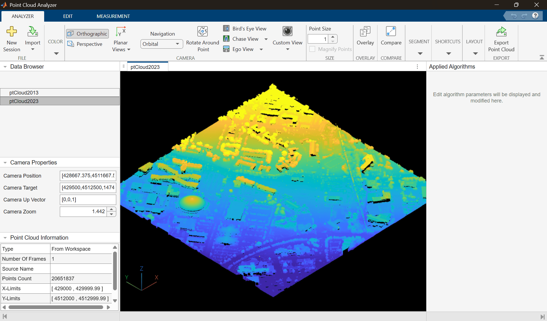
To import the point clouds, on the app toolstrip, select Import > From Workspace. In the Import From Workspace dialog box, select ptCloud2013 and ptCloud2023, then click OK. Both point clouds appear in the Data Browser pane. The app displays the last imported point cloud (ptCloud2023) in the visualization pane.

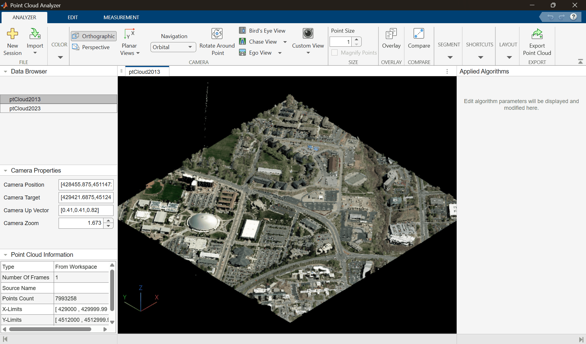
To view the other point cloud, ptCloud2013, select it in the Data Browser pane.

Preprocess Point Clouds

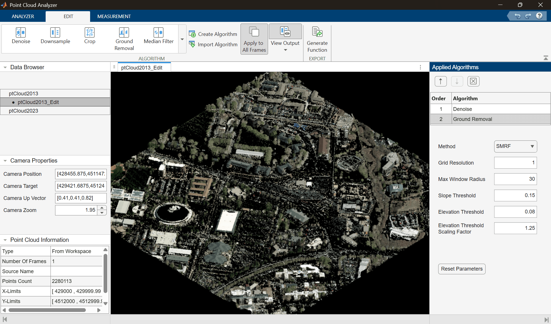
Before comparing the point clouds, remove noise and ground points from both point clouds.

1. In the Data Browser, select ptCloud2013.

2. To denoise the point cloud, from the app toolstrip, select Edit tab and then select Denoise from the Algorithm section. In the Applied Algorithms pane, set the Number of Nearest Neighbors to 15 and Outlier Threshold to 1.

3. From the Algorithms section on the app toolstrip, select Ground Removal. Set Max Window Radius to 30 and Elevation Threshold to 0.08.

4. Repeat steps 1-3 for the ptCloud2023 point cloud.

These parameter values are specific to this data set and might require adjustment for other point clouds. After preprocessing, both point clouds contain only the above-ground structures — buildings, trees, and other elevated objects. Depending on your application, use any combination of built-in algorithms such as Denoise, Downsample, Crop, or Ground Removal. To apply custom preprocessing, use the Custom Function option in the Edit tab.

Overlay Point Clouds

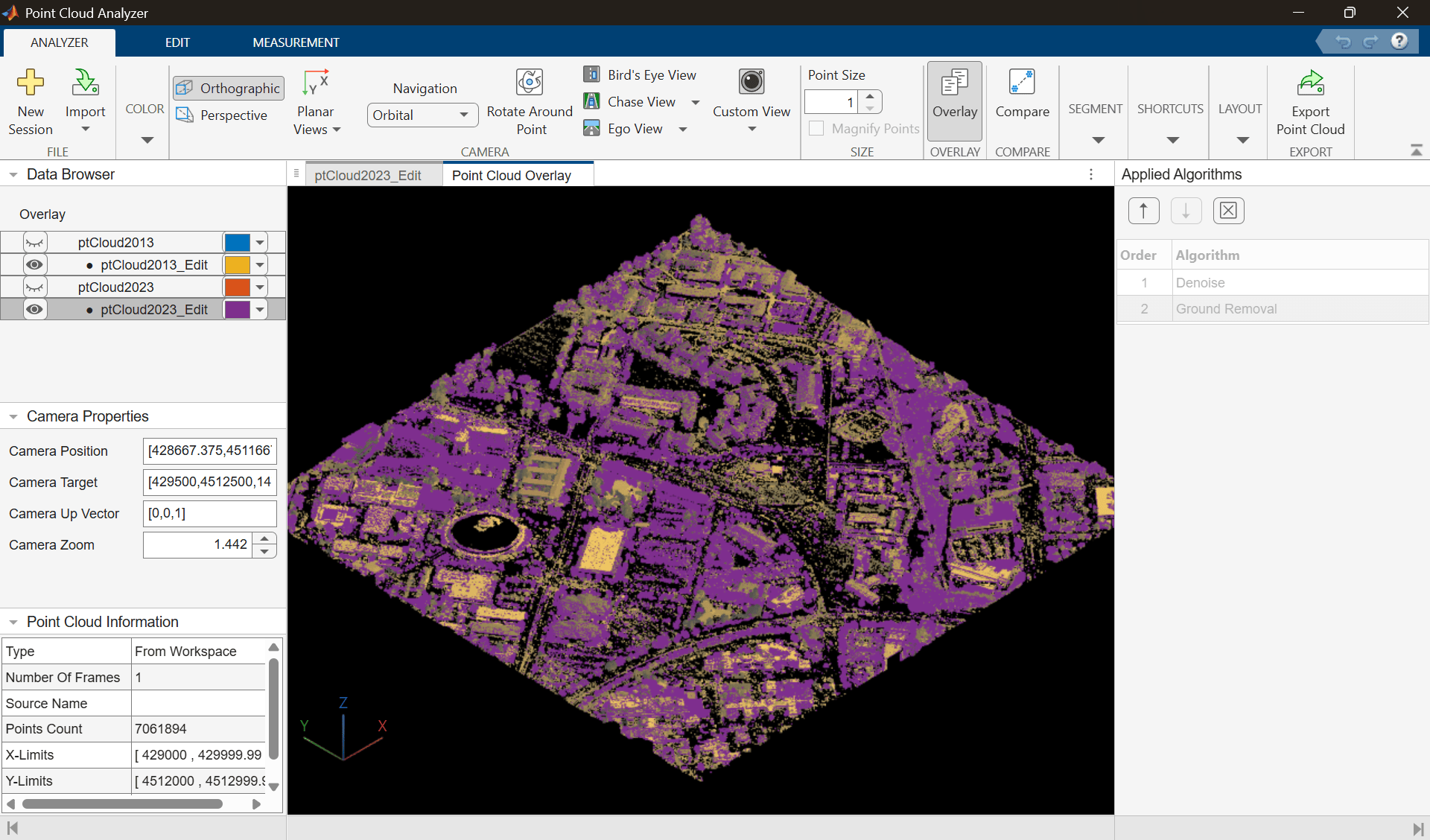
To inspect spatial differences between the point clouds, overlay them in the same view.

1. On the app toolstrip, select Analyzer tab, and then select Overlay.

2. In the Data Browser pane, turn off the visibility of ptCloud2013 and ptCloud2023 so that only the edited point clouds are displayed.

In the overlay view, observe areas where structures appear in one point cloud but not the other.

Compare Point Clouds

To quantify differences between the two point clouds, compute distances using the Compare feature.

1. On the app toolstrip, select Compare. The app opens the Compare tab and displays an empty Point Cloud Difference view.

2. In the Compare tab, set the Reference point cloud to ptCloud2013_Edit.

3. Set the Target point cloud to ptCloud2023_Edit.

4. Select Location as the comparison Attribute.

5. Click Calculate Difference.

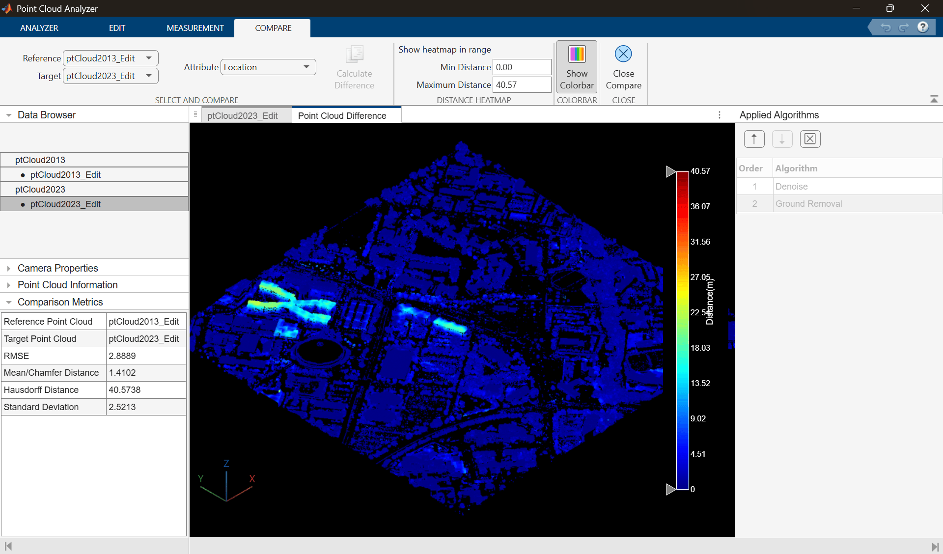
The Location attribute computes the Euclidean distance from each point in the target point cloud to its closest point in the reference point cloud. Because the ground has been removed, this captures changes in above-ground structures over the 10-year period.

Interpret Distance Heatmap

To interpret differences between the point clouds, use the distance heatmap shown in the Point Cloud Difference view. The colorbar maps colors to distance values:

• Blue regions — Areas with minimal or no change between the two point clouds.

• Green/Yellow regions — Areas with moderate changes, such as building renovations.

• Orange/Red regions — Areas with significant changes, such as new construction or demolished buildings.

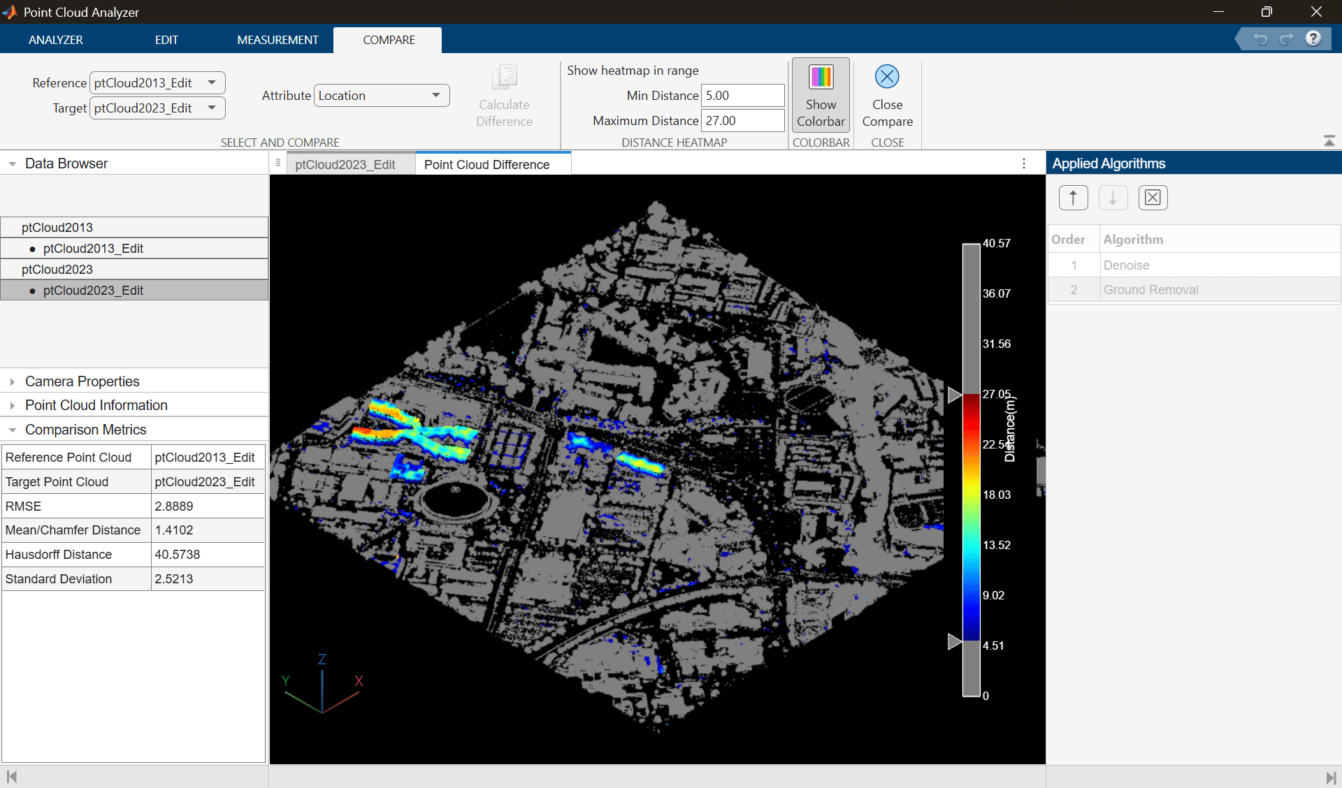
You can adjust the minimum and maximum distance values or move the colorbar markers to focus on specific distance ranges. Setting a minimum threshold of 5 m helps suppress minor surface variations and highlight larger structural differences. Setting a maximum threshold of 27 m excludes extreme outliers and focuses the color gradient on building-scale changes. Points in the selected range are colored according to the heatmap, while points outside the range appear in their original color or in gray if color information is not available.

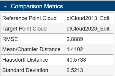
To further interpret differences between the point clouds, review the comparison metrics in the Comparison Metrics pane. Examine summary statistics such as RMSE, maximum, and mean distance values to understand the overall magnitude and spread of geometric differences.

For this data set, the metrics indicate:

• A moderate RMSE and Chamfer distance — most of the scene remains unchanged, with localized structural differences from new construction and demolitions.

• A high standard deviation — changes concentrate in specific areas instead of occurring uniformly across the scene.

• A large Hausdorff distance — tall new structures in one survey have no close match in the other, resulting in the large distance.

References

[1] USGS Lidar Point Cloud UT_Wasatch_L4_2013 courtesy of the U.S. Geological Survey.

[2] USGS Lidar Point Cloud UT_2023_SaltLakeCo_1_C24 courtesy of the U.S. Geological Survey.