Create a Digital Twin of a TI mmWave Radar Operating in DDM Mode

R2026b

Since R2026b

This example uses:

Radar Toolbox Support Package for Texas Instruments mmWave Radar Sensors Radar Toolbox Support Package for Texas Instruments mmWave Radar Sensors
Radar Toolbox Radar Toolbox
Sensor Fusion and Tracking Toolbox Sensor Fusion and Tracking Toolbox

This example shows you how to create a waveform-level digital twin of a Texas Instruments™ (TI) AWR2944EVM mmWave radar operating in Doppler Division Multiplexing (DDM) mode. A digital twin enables algorithm development, performance evaluation, and what-if analysis without requiring physical hardware or a controlled test environment. The example uses a radar configuration file to configure custom RF cascade components and simulate a DDM MIMO radar with simultaneous transmission from all transmit antennas in MATLAB®.

The workflow includes custom models for DDM phase coding, waveform generation, signal propagation, dechirp processing, range-Doppler estimation, CFAR detection, and beamforming using an L-shaped virtual array. The example also compares synthetic data generated by the model with data collected from the physical radar. The results show close agreement between the real sensor and its digital twin.

The Radar Toolbox™ Support Package for Texas Instruments mmWave Radar Sensors enables the collection of I/Q data from TI mmWave radar devices, as demonstrated in I/Q Data Collection and Detection Generation with Texas Instruments (TI) millimeter-wave (mmWave) Radar. This example extends that workflow by showing how to create an accurate model of the AWR2944EVM DDM radar using the radarTransceiver System object™.

By creating a waveform-level model, you can develop and test DDM processing algorithms in custom scenarios without the cost and complexity of physical test environments. The processing workflow in this example follows these steps:

Parse the configuration file
Build the radar model
Simulate DDM signals
Perform range-Doppler processing
Detect targets
Estimate angles
Compare with real-world data.

This example uses an AWR2944EVM radar connected to a DCA1000EVM data capture board. Together, these boards stream raw ADC samples that you can process and visualize using MATLAB functions and System objects.

DDM Compared With TDM

In Time Division Multiplexing (TDM), only one transmit antenna is active during each chirp. This simplifies signal processing but reduces the maximum unambiguous velocity by the number of transmit antennas.

In Doppler Division Multiplexing (DDM), all transmit antennas are active during every chirp. Each antenna applies a unique phase progression:

$ϕ_{T X_{k}} (m) = e^{j 2 π \cdot phaseOrder (k) \cdot m / N_{s u b}}$

where $k$ is the TX index, $m$ is the chirp number, and $N_{s u b}$ is the number of subbands.

This phase coding creates orthogonal signals that separate into distinct Doppler subbands after Doppler processing. Compared with TDM, DDM provides several advantages:

Preserves the full maximum unambiguous velocity.
Improves signal-to-noise ratio (SNR) because all transmit antennas contribute to every chirp.
Maintains the same virtual array size (4 TX × 4 RX = 16 virtual elements).

The primary trade-off is increased signal-processing complexity. DDM requires additional Doppler-domain processing to separate the contributions from each transmit antenna. Because each transmitter occupies a dedicated Doppler subband, the available unambiguous velocity range for each transmit antenna is reduced relative to the overall Doppler span.

DDM Subband Demodulation

After performing a Doppler FFT across all chirps in a frame, the Doppler spectrum is divided into $N_{s u b}$ equal-width subbands.

Each transmit antenna produces a target response in a unique subband. The response is offset from the base Doppler bin by:

$d_{k} = d_{b a s e} + p h a s e O r d e r (k) N_{s u b s i z e}$

where

$d_{k}$ = Doppler-bin location of TX antenna $k$
$d_{b a s e}$ = Doppler bin corresponding to the target's actual velocity
$p h a s e O r d e r (k)$ = DDM phase-order index assigned to TX antenna $k$
$N_{s u b s i z e}$ = width of each Doppler subband in bins

The AWR2944EVM DDM configuration uses six subbands. Four subbands correspond to the four active transmit antennas, while two remain unused.

Assumptions

This model makes the following assumptions:

All four transmit and four receive channels are enabled.
Every chirp uses the same linear frequency-modulated (LFM) waveform.
Target velocity remains constant within a frame.
DDM phase coding follows the ddmPhaseShiftAntOrder field in the configuration file, and uses the same antenna ordering as antGeometryCfg.
Antenna element patterns are approximated using a cosine response that matches the AWR2944EVM beamwidth specification.
Signal propagation occurs in free space, with no multi-path reflections or clutter.

Model the Radar Transceiver from the Configuration File

Read the Configuration File

To operate the AWR2944EVM in DDM mode, you must provide a configuration file that defines the waveform, antenna configuration, and DDM parameters. The MMWAVE SDK User Guide describes the configuration file format and associated commands.

The remainder of this example uses the configuration file shown below:

type("AWR294X_profile_DDM_DCA.cfg")

% ***************************************************************
% Created for SDK ver:04.07
% Created using Visualizer ver:4.7.0.0
% Frequency:76
% Platform:AWR294X
% Scene Classifier:best_range_res
% Azimuth Resolution(deg):3Azim + Elevation
% Range Resolution(m):0.174
% Maximum unambiguous Range(m):8.91
% Maximum Radial Velocity(m/s):1.9
% Radial velocity resolution(m/s):0.04
% Frame Duration(msec):100
% RF calibration data:None
% Range Detection Threshold (dB):15
% Doppler Detection Threshold (dB):15
% Range Peak Grouping:disabled
% Doppler Peak Grouping:disabled
% Angle of Arrival FoV: Full FoV
% Range FoV: Full FoV
% Doppler FoV: Full FoV
% ***************************************************************
sensorStop
flushCfg
dfeDataOutputMode 1
channelCfg 15 15 0
adcCfg 2 0
adcbufCfg -1 1 1 0 1
lowPower 0 0
profileCfg 0 76 494 2.5 25 0 0 40 1 64 2976 0 0 30
chirpCfg 0 5 0 0 0 0 0 15
frameCfg 0 5 16 0 64 100 1 0
lowPower 0 0
guiMonitor -1 1 1 0 0 0 1
antGeometryCfg 1 0 1 1 1 2 1 3 0 2 0 3 0 4 0 5 1 4 1 5 1 6 1 7 1 8 1 9 1 10 1 11 0.5 0.8
cfarCfg -1 0 3 16 0 0 1 15 0 7 0 1
cfarCfg -1 1 3 16 0 0 1 15 0 7 0 1
compressionCfg -1 1 0 0.5 8
intfMitigCfg -1 15 18
localMaxCfg -1 6 40
ddmPhaseShiftAntOrder 0 2 3 1
antennaCalibParams 0 1 0 1 0 1 0 1 0 1 0 1 0 1 0 1 0 1 0 1 0 1 0 1 0 1 0 1 0 1 0 1
measureRangeBiasAndRxChanPhase 0 1.5 0.2
aoaFovCfg -1 -90 90 -90 90
calibData 0 0 0
lvdsStreamCfg -1 0 1 0
sensorStart

Many configuration commands are required to initialize the radar but are not relevant to waveform-level modeling. To create an accurate model, only a subset of parameters and datasheet specifications are needed. The following configuration entries are relevant to the DDM model:

Line Header	Description
profileCfg	Waveform and ADC properties, including start frequency, sweep slope, number of samples, and sample rate
frameCfg	Chirp configuration, frame structure, and frame rate
channelCfg	Active transmit and receive channels
ddmPhaseShiftAntOrder	DDM subband assignment for each transmit antenna
antGeometryCfg	Virtual antenna array geometry (L-shaped, 16 elements)
cfarCfg	CFAR detection parameters

For more information, refer to these links:

Manually extracting these parameters requires cross-referencing several sections of the SDK documentation. To simplify this process, the example provides the helper class helperParseDDMConfig in the tiRadar folder. The helper class extracts the configuration values required by the waveform-level model.

addpath("tiRadar")
radarCfg = helperParseDDMConfig("AWR294X_profile_DDM_DCA.cfg")

radarCfg = struct with fields:
                   numRx: 4
                   numTx: 4
             numSubbands: 6
           ddmPhaseOrder: [0 2 3 1]
               startFreq: 7.6000e+10
                idleTime: 4.9400e-04
            adcStartTime: 2.5000e-06
             rampEndTime: 2.5000e-05
               freqSlope: 4.0000e+13
           numADCSamples: 64
           adcSampleRate: 2976000
                rxGaindB: 30
           numChirpTypes: 6
                numLoops: 16
       numChirpsPerFrame: 96
             framePeriod: 0.0640
          chirpCycleTime: 5.1900e-04
         sampledRampTime: 2.1505e-05
               bandwidth: 8.6022e+08
              centerFreq: 7.6530e+10
                  lambda: 0.0039
         CenterFrequency: 7.6530e+10
               Bandwidth: 8.6022e+08
              SweepSlope: 4.0000e+13
           ADCSampleRate: 2976000
         SampledRampTime: 2.1505e-05
         SamplesPerChirp: 64
               NumChirps: 96
         NumTransmitters: 4
            NumReceivers: 4
                     PRF: 1.9268e+03
                  RxGain: 30
            rangeFFTSize: 64
            numRangeBins: 32
                rangeRes: 0.1743
            rangeBinSize: 0.1743
                maxRange: 5.0185
               rangeGrid: [0 0.1743 0.3485 0.5228 0.6970 0.8713 1.0455 1.2198 1.3940 1.5683 1.7425 1.9168 2.0911 2.2653 2.4396 2.6138 2.7881 2.9623 3.1366 3.3108 3.4851 3.6593 3.8336 4.0079 4.1821 4.3564 4.5306 4.7049 4.8791 5.0534 5.2276 5.4019]
          numDopplerBins: 96
          dopplerFFTSize: 96
             maxVelocity: 1.8870
             subbandSize: 16
                  velRes: 0.0393
      maxSubbandVelocity: 0.3145
    numOutputDopplerBins: 16
             dopplerGrid: [-0.3145 -0.2752 -0.2359 -0.1966 -0.1572 -0.1179 -0.0786 -0.0393 0 0.0393 0.0786 0.1179 0.1572 0.1966 0.2359 0.2752]
             antGeometry: [1×1 struct]
      numVirtualAntennas: 16
       azimuthAntennaIdx: [1 2 3 4 9 10 11 12 13 14 15 16]
     elevationAntennaIdx: [5 6 7 8]
      numAzimuthAntennas: 12
    numElevationAntennas: 4
             calibVector: [16×1 double]
               rangeCFAR: [1×1 struct]
             dopplerCFAR: [1×1 struct]
      compressionEnabled: 1
           azimuthLimits: [-90 90]
         elevationLimits: [-90 90]
                     prf: 1.9268e+03
               dutyCycle: 0.0414
                 cfgFile: "AWR294X_profile_DDM_DCA.cfg"

The helper class assumes a DDM configuration in which all four transmit antennas operate simultaneously with unique phase codes. It uses ddmPhaseShiftAntOrder to determine phase assignments and antGeometryCfg to construct the virtual array. The parser also assumes that all receive channels are enabled.

Modify the parser if you need to support additional radar configurations or optional features.

After parsing the configuration file, use the helperDDMRadarAndProcessor class to create the radar transceiver and associated signal-processing components. This class serves the same purpose as helperRadarAndProcessor in the TDM digital twin example (Create a Digital Twin of a TI mmWave Radar).

radarSystem = helperDDMRadarAndProcessor(radarCfg)

radarSystem = 
  helperDDMRadarAndProcessor with properties:

              RadarTransceiver: [1×1 radarTransceiver]
                  VirtualArray: [1×1 phased.ConformalArray]
                            Fc: 7.6530e+10
                            Fs: 8.6022e+08
    NumSamplesDuringPulseWidth: 18499
         RangeDopplerProcessor: [1×1 phased.RangeResponse]
                    TwoDimCFAR: [1×1 phased.CFARDetector2D]
                     DDMSwitch: [1×1 helperDDMSwitch]
                    PhaseCoder: [1×1 helperDDMPhaseCoder]
                  PhaseShiftBf: [1×1 phased.PhaseShiftBeamformer]

The radar transceiver is available through the RadarTransceiver property. The following sections describe how the radarTransceiver System object is configured to replicate the behavior of the AWR2944EVM.

radarSystem.RadarTransceiver

ans = 
  radarTransceiver with properties:

                Waveform: [1×1 phased.LinearFMWaveform]
             Transmitter: [1×1 phased.Transmitter]
         TransmitAntenna: [1×1 phased.Radiator]
          ReceiveAntenna: [1×1 phased.Collector]
                Receiver: [1×1 phased.Receiver]
      MechanicalScanMode: 'None'
      ElectronicScanMode: 'None'
        MountingLocation: [0 0 0]
          MountingAngles: [0 0 0]
    NumRepetitionsSource: 'Property'
          NumRepetitions: 96
       RangeLimitsSource: 'Property'
             RangeLimits: [0 Inf]
         RangeOutputPort: false
          TimeOutputPort: false

Configure the Antennas

Antenna Arrays

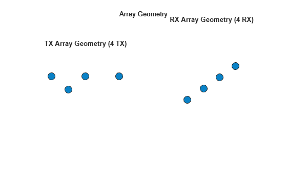
The AWR2944EVM includes four transmit antennas and four receive antennas. In DDM mode, all transmit antennas are active during every chirp and apply distinct phase progressions.

The antenna locations are derived directly from the antGeometryCfg entry in the configuration file.

figure;
subplot(1,2,1)
viewArray(radarSystem.RadarTransceiver.TransmitAntenna.Sensor, ...
    'ShowLocalCoordinates', false, 'ShowAnnotation', false)
title('TX Array Geometry (4 TX)')
subplot(1,2,2)
viewArray(radarSystem.RadarTransceiver.ReceiveAntenna.Sensor, ...
    'ShowLocalCoordinates', false, 'ShowAnnotation', false)
title('RX Array Geometry (4 RX)')

Figure contains 2 axes objects. Hidden axes object 1 with title TX Array Geometry (4 TX) contains an object of type scatter. Hidden axes object 2 with title RX Array Geometry (4 RX) contains an object of type scatter.

Virtual Array

The combination of four transmit antennas and four receive antennas forms a 16-element virtual array. The virtual array geometry is identical to the geometry used in TDM radar systems.

The L-shaped array provides:

12 azimuth elements with half-wavelength spacing.
4 elevation elements.

Unlike TDM, DDM maintains this virtual aperture without reducing the maximum unambiguous Doppler velocity. For more information about creating large virtual arrays, see Simulate an Automotive 4D Imaging MIMO Radar.

figure;
viewArray(radarSystem.VirtualArray)
title('Virtual Array (L-shaped, 16 elements)')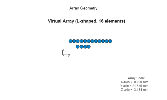

Figure contains an axes object. The hidden axes object with title Virtual Array (L-shaped, 16 elements), xlabel x axis (Az 0 El 0) -->, ylabel y axis --> contains 7 objects of type scatter, line, text.

Antenna Elements

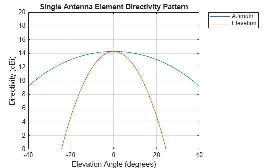
Both the transmit and receive arrays use the phased.CosineAntennaElement System object™. This element approximates the directivity pattern specified in the AWR2944EVM datasheet.

For more accurate antenna modeling, use phased.CustomAntennaElement and provide measured or datasheet-derived antenna patterns.

element = radarSystem.RadarTransceiver.TransmitAntenna.Sensor.Element;

Plot the Pattern

figure;
az = -180:180;
el = 0;
pattern(element, radarCfg.centerFreq, az, el, CoordinateSystem="rectangular", Type='directivity');
hold on;
az = 0;
el = -90:90;
pattern(element, radarCfg.centerFreq, az, el, CoordinateSystem="rectangular", Type='directivity');
legend('Azimuth','Elevation')
title('Single Antenna Element Directivity Pattern')
xlim([-40 40])
ylim([0 20])

Figure contains an axes object. The axes object with title Single Antenna Element Directivity Pattern, xlabel Elevation Angle (degrees), ylabel Directivity (dBi) contains 2 objects of type line. These objects represent Azimuth, Elevation.

Transmitter

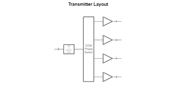
The transmitter uses a cascade configuration that models three key aspects of AWR2944EVM DDM operation:

Signal splitting for de-chirping.
DDM phase coding across transmit antennas.
Transmit power amplification.

These components are implemented using the cascade transmitter architecture shown below.

figure
viewLayout(radarSystem.RadarTransceiver.Transmitter)

Figure contains an axes object. The hidden axes object with title Transmitter Layout contains 23 objects of type line, text.

Signal Splitter

The radar performs dechirp processing by mixing received echoes with a copy of the transmitted waveform. The signal splitter provides this waveform copy for the receiver mixer.

DDM Phase Switch

The helperDDMSwitch System object applies DDM phase coding to all transmit channels.

Unlike TDM, in which only one transmitter is active per chirp, DDM activates all transmitters simultaneously. For chirp m, transmit antenna k receives the following phase shift: $e^{j 2 π \cdot phaseOrder (k) \cdot m / 6}$

The configuration line [ddmPhaseShiftAntOrder 0 2 3 1] assigns a unique Doppler subband to each transmit antenna. For a 96-bin Doppler spectrum divided into six subbands, each subband contains 16 Doppler bins.

Transmit Power

Each transmit channel operates at 13.5 dBm, as specified in the AWR2944EVM datasheet.

Because all four transmit antennas radiate simultaneously, total transmitted power is approximately 6 dB greater than a single-transmitter TDM configuration. The model represents this power level using a saturated power amplifier.

transmitPower = radarSystem.RadarTransceiver.Transmitter.Cascade{3}.OPsat % dBm

transmitPower = 
13.5000

Receiver

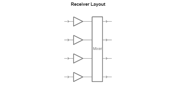
The receiver model includes both low-noise amplification and dechirp mixing.

figure
viewLayout(radarSystem.RadarTransceiver.Receiver)

Figure contains an axes object. The hidden axes object with title Receiver Layout contains 26 objects of type line, text.

Low Noise Amplifier

The receiver first applies gain and noise figure characteristics that match the AWR2944EVM front end.

Receiver gain is obtained from the radar configuration file. The noise figure is set to 12 dB according to the AWR2944EVM datasheet.

The model uses an rf.Amplifier object with noise enabled to represent the low-noise amplifier (LNA).

LNA = radarSystem.RadarTransceiver.Receiver.Cascade{1};
rxGain = LNA.Gain

rxGain = 
30

noiseFigure = LNA.NF

noiseFigure = 
12

Mixer

The mixer performs de-chirping by multiplying the received echo with a copy of the transmitted waveform.

This operation converts the high-bandwidth FMCW signal into a lower-frequency intermediate-frequency (IF) signal that encodes target range information. De-chirping provides a computationally efficient alternative to matched filtering and reduces receiver bandwidth requirements.

Waveform

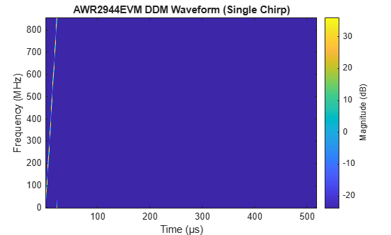
The AWR2944EVM transmits a linear frequency-modulated (LFM) chirp waveform.

Although both phased.LinearFMWaveform and phased.FMCWWaveform can generate chirp signals, only phased.LinearFMWaveform supports duty cycles below 100%.

According to the configuration file, a chirp repeats every 519 μs, while the sampled ramp occupies only 21.5 μs. As a result, the waveform duty cycle is approximately 4%.

In other words, the radar actively transmits for only about 4% of each pulse repetition interval (PRI).

PRI = 1/radarCfg.PRF

PRI = 
5.1900e-04

sampledRampTime = radarCfg.sampledRampTime

sampledRampTime = 
2.1505e-05

dutyCycle = sampledRampTime/PRI

dutyCycle = 
0.0414

Configure the LFM waveform so that the transmit ramp duration equals the sampled ramp time. The remaining portion of the PRI contains no transmitted signal.

figure
stft(radarSystem.RadarTransceiver.Waveform(), radarSystem.Fs, 'FrequencyRange', 'twosided')
title('AWR2944EVM DDM Waveform (Single Chirp)')

Figure contains an axes object. The axes object with title AWR2944EVM DDM Waveform (Single Chirp), xlabel Time (μs), ylabel Frequency (MHz) contains an object of type image.

Sampling Rate

The physical radar includes an analogue front end that converts received reflections to an intermediate frequency before digitization. This architecture allows the hardware ADC to sample at 2.976 Msps rather than at the waveform bandwidth.

The software model operates differently. It first generates a full-bandwidth waveform at approximately 860 MHz, propagates the signal through the environment, and then performs digital de-chirping. After de-chirping, the IF signal is downsampled to match the ADC sampling rate using the downsampleIF method.

Number of Chirps

Each DDM frame contains 96 chirps, consisting of 6 chirp types repeated over 16 loops. Depending on your application, you can configure the number of chirps in one of the following ways:

When analyzing the waveform object independently, set the NumPulses property of the waveform System object.
For most applications where target velocity remains constant within a frame, set the NumRepetitions property of the radarTransceiver object to the desired number of chirps.
For scenarios that require target motion updates between chirps, such as simulations that use backscatterPedestrian, set NumRepetitions to one and update the target state within a loop.

The DDM phase switch maintains its internal chirp counter across repetitions, ensuring that the correct phase code is applied to each chirp.

fprintf('Full-bandwidth sample rate: %.2f MHz\n', radarSystem.Fs/1e6);

Full-bandwidth sample rate: 860.22 MHz

fprintf('Samples per chirp (full BW): %d\n', radarSystem.NumSamplesDuringPulseWidth);

Samples per chirp (full BW): 18499

fprintf('Samples per chirp (ADC):     %d\n', radarCfg.numADCSamples);

Samples per chirp (ADC):     64

fprintf('Decimation factor:           %d\n', ...
    round(radarSystem.NumSamplesDuringPulseWidth / radarCfg.numADCSamples));

Decimation factor:           289

Data Processing

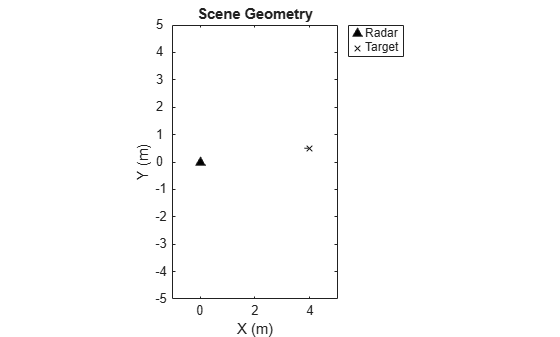
To evaluate how the AWR2944EVM model detects a point target, define a target with a specified position and velocity. The radar model automatically accounts for motion-induced phase changes between chirps. Therefore, set the number of radar repetitions to match the number of chirps in the frame.

radarSystem.RadarTransceiver.NumRepetitions = radarCfg.numChirpsPerFrame;
tgt1 = struct('Position', [4 0.5 0], 'Velocity', [-0.2 0 0], 'RCS', 5);

Display the simulated radar scene to verify the target geometry.

tp = theaterPlot('XLim', [-1 5], 'YLim', [-5 5]);
radarPlotter = platformPlotter(tp, 'DisplayName', 'Radar', 'Marker', '^', 'MarkerFaceColor', 'k');
targetPlotter = platformPlotter(tp, 'DisplayName', 'Target', 'Marker', 'x');
plotPlatform(radarPlotter, [0 0 0])
plotPlatform(targetPlotter, tgt1.Position, tgt1.Velocity)
title('Scene Geometry')

Figure contains an axes object. The axes object with title Scene Geometry, xlabel X (m), ylabel Y (m) contains 2 objects of type line. One or more of the lines displays its values using only markers These objects represent Radar, Target.

Next, simulate waveform transmission and reception. The radarTransceiver object generates a full-bandwidth chirp, applies DDM phase coding, propagates the signal to the target, and performs dechirp mixing on reception.

After de-chirping, retain only the active portion of the signal and downsample it to match the ADC sample rate. The resulting data cube has dimensions [(samples per chirp) x channels x (chirps per frame)].

reset(radarSystem.DDMSwitch);
if isLocked(radarSystem.RadarTransceiver)
    release(radarSystem.RadarTransceiver);
end

targets = struct('Position', tgt1.Position(:).', ...
    'Velocity', tgt1.Velocity(:).', ...
    'Signatures', {{rcsSignature('Pattern', tgt1.RCS)}});
time = 0;
sig = radarSystem.RadarTransceiver(targets, time);
sig = radarSystem.downsampleIF(sig);
size(sig)

ans = 1×3

    64    4    96

Range Doppler Processing

Use the boresightRD method to compute the DDM range-Doppler response. This method performs the following processing steps:

Applies a range FFT to each chirp using a Hann window and retains only the positive-frequency half of the spectrum.
Applies a Doppler FFT across all 96 chirps using a Hann window.
Performs DDM subband extraction by dividing the 96-bin Doppler spectrum into six subbands of 16 bins each. The four active transmit antenna subbands are extracted according to phaseOrder(k) × subbandSize, and their power is summed non-coherently.
Sums power non-coherently across the four receive channels, providing approximately 12 dB of integration gain.

The output is a 32-by-16 range-Doppler map containing 32 range bins and 16 Doppler bins per subband.

[rgdp, rngBins, dpBins] = radarSystem.boresightRD(sig);

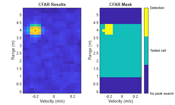
CFAR Detection

Use the findPeaksRangeDoppler method to perform two-dimensional ordered-statistics constant false alarm rate (OS-CFAR) detection.

The detector uses circular Doppler padding to handle velocity wraparound and applies a local maximum filter in range to consolidate nearby detections.

Experiment with different CFAR parameter values and observe how the detection results change.

[cfarMask, peakLocations] = radarSystem.findPeaksRangeDoppler(rgdp);
radarSystem.cfarPlotter(rgdp, cfarMask, peakLocations, rngBins, dpBins)

Figure contains 2 axes objects. Axes object 1 with title CFAR Results, xlabel Velocity (m/s), ylabel Range (m) contains 2 objects of type image, scatter. Axes object 2 with title CFAR Mask, xlabel Velocity (m/s), ylabel Range (m) contains an object of type image.

Angle Processing

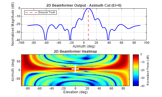
Estimate target angles using DDM subband demodulation and two-dimensional beamforming.

For a target detected at Doppler bin d, the algorithm performs the following steps:

Computes the base FFT bin corresponding to the detected velocity.
Locates the contribution from each transmit antenna $k$ at the Doppler bin associated with its DDM phase assignment: $(d + phaseOrder (k) \times 16) m o d 96$
Combines each transmit channel with all receive channels to form a 16-element virtual antenna vector.
Applies the antenna calibration vector obtained from the configuration file.
Performs two-dimensional phase-shift beamforming to estimate azimuth and elevation.

[bfOut, azScan, elScan] = radarSystem.getBfAngleOutput(sig, peakLocations);

Plot the beamforming output.

helperPlotBfOutput(bfOut, tgt1, azScan, elScan)

Azimuth Beamforming Using the 12-Element Sub-Array

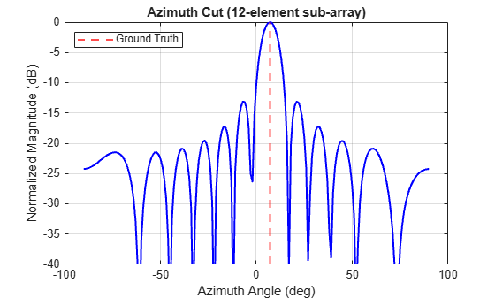
The L-shaped virtual array contains 12 elements along the azimuth axis. This subarray provides higher azimuth resolution than the full two-dimensional scan.

Compute and display the azimuth beamforming response using the azimuth subarray.

[azEst, bfAzOutput] = radarSystem.getBfAzimuthOutput(sig, peakLocations);

figure;
bfAzdB = mag2db(bfAzOutput + eps);
bfAzNorm = bfAzdB - max(bfAzdB);
plot(azScan, bfAzNorm, 'b-', 'LineWidth', 1.5);
hold on;
tgtAz = atan2d(tgt1.Position(2), tgt1.Position(1));
gt = xline(tgtAz, 'r--', 'LineWidth', 1.5);
hold off;
xlabel('Azimuth Angle (deg)')
ylabel('Normalized Magnitude (dB)')
title(sprintf('Azimuth Cut (%d-element sub-array)', radarCfg.numAzimuthAntennas))
legend(gt, 'Ground Truth', 'Location', 'northwest')
grid on;
ylim([-40 0])

Figure contains an axes object. The axes object with title Azimuth Cut (12-element sub-array), xlabel Azimuth Angle (deg), ylabel Normalized Magnitude (dB) contains 2 objects of type line, constantline. This object represents Ground Truth.

Detection Summary

Compare the detected target parameters with the ground-truth target values.

The results show close agreement between the estimated and true target parameters. The observed errors are substantially smaller than the range and Doppler bin resolutions, indicating that the processing chain accurately recovers the target location, velocity, and azimuth angle.

fprintf('\n--- Detection Results ---\n');

--- Detection Results ---

for d = 1:size(peakLocations, 2)
    rb = peakLocations(1, d);
    db = peakLocations(2, d);
    detRange = rngBins(rb);
    detVel = dpBins(db);
    fprintf('Detection %d: Range = %.3f m, Velocity = %.3f m/s, Azimuth = %.1f deg\n', ...
        d, detRange, detVel, azEst(d));
end

Detection 1: Range = 4.008 m, Velocity = -0.197 m/s, Azimuth = 7.0 deg

fprintf('\n--- Ground Truth ---\n');

--- Ground Truth ---

trueRange = norm(tgt1.Position);
trueVel = dot(tgt1.Velocity, tgt1.Position) / trueRange;
trueAz = atan2d(tgt1.Position(2), tgt1.Position(1));
fprintf('Target: Range = %.3f m, Velocity = %.3f m/s, Azimuth = %.1f deg\n', ...
    trueRange, trueVel, trueAz);

Target: Range = 4.031 m, Velocity = -0.198 m/s, Azimuth = 7.1 deg

fprintf('\n--- Errors ---\n');

--- Errors ---

if ~isempty(peakLocations)
    fprintf('Range error:    %+.3f m (< 1 range bin = %.3f m)\n', ...
        rngBins(peakLocations(1,1)) - trueRange, radarCfg.rangeRes);
    fprintf('Velocity error: %+.3f m/s (< 1 Doppler bin = %.4f m/s)\n', ...
        dpBins(peakLocations(2,1)) - trueVel, radarCfg.velRes);
    fprintf('Azimuth error:  %+.1f deg\n', azEst(1) - trueAz);
end

Range error:    -0.023 m (< 1 range bin = 0.174 m)

Velocity error: +0.002 m/s (< 1 Doppler bin = 0.0393 m/s)

Azimuth error:  -0.1 deg

Radar Performance

The selected DDM configuration produces the following radar performance characteristics.

Unlike TDM, DDM preserves the full maximum unambiguous velocity because all transmit antennas operate simultaneously. The maximum unambiguous velocity is therefore equal to $λ \cdot P R F / 4$ and is not reduced by the number of transmit antennas.

Velocity resolution is determined by the Doppler-bin spacing within each subband and is given by $v_{m a x} / (N_{s u b_s i z e} / 2)$ .

The following measurements summarize the key radar performance metrics for this configuration.

fprintf('\n=== AWR2944EVM DDM Radar Performance (DCA Config) ===\n');

=== AWR2944EVM DDM Radar Performance (DCA Config) ===

fprintf('  Range resolution:       %.3f m (c/2B)\n', radarCfg.rangeRes);

  Range resolution:       0.174 m (c/2B)

fprintf('  Velocity resolution:    %.4f m/s\n', radarCfg.velRes);

  Velocity resolution:    0.0393 m/s

fprintf('  Max unambiguous range:  %.1f m\n', radarCfg.maxRange);

  Max unambiguous range:  5.0 m

fprintf('  Max unambiguous vel:    %.2f m/s (full, not reduced by N_TX)\n', radarCfg.maxVelocity);

  Max unambiguous vel:    1.89 m/s (full, not reduced by N_TX)

fprintf('  Subband velocity:       +/-%.3f m/s (per TX subband)\n', radarCfg.maxSubbandVelocity);

  Subband velocity:       +/-0.314 m/s (per TX subband)

fprintf('  Frame rate:             %.1f Hz\n', 1/radarCfg.framePeriod);

  Frame rate:             15.6 Hz

fprintf('  Subbands:               %d (%d active + 2 empty)\n', radarCfg.numSubbands, radarCfg.numTx);

  Subbands:               6 (4 active + 2 empty)

fprintf('  DDM TX coding gain:     %.1f dB over single-TX\n', 10*log10(radarCfg.numTx));

  DDM TX coding gain:     6.0 dB over single-TX

fprintf('  Integration gain:       +%.1f dB (4TX x 4RX)\n', 10*log10(radarCfg.numTx*radarCfg.numRx));

  Integration gain:       +12.0 dB (4TX x 4RX)

Compare Synthetic and Real-World Data

This section compares synthetic data generated by the digital twin with data collected from a real AWR2944EVM radar.

To acquire the real-world dataset, the AWR2944EVM was configured using the same DDM configuration described earlier in this example. During data collection, a corner reflector moved toward the radar.

A recording captured with the DCA1000EVM serves as a reference dataset for validating the digital twin. The recording contains a corner reflector located approximately 1.9 m from the radar and moving toward it at 0.275 m/s, corresponding to approximately seven Doppler bins. The target remains near boresight throughout the measurement.

To create a comparable synthetic scenario, define a point target with the same position and velocity. Applying identical processing to both datasets enables a direct comparison between simulation and hardware measurements.

Synthetic Data

Define a corner-reflector target and generate a synthetic radar data cube using the digital twin.

tgt2 = struct('Position', [1.917 0 0], 'Velocity', [-0.275 0 0], ...
    'Signatures', {{rcsSignature('Pattern', 5)}});
reset(radarSystem.DDMSwitch);
if isLocked(radarSystem.RadarTransceiver)
    release(radarSystem.RadarTransceiver);
end
radarSystem.RadarTransceiver.NumRepetitions = radarCfg.numChirpsPerFrame;
sigSynthetic = radarSystem.RadarTransceiver(tgt2, 0);
sigSynthetic = radarSystem.downsampleIF(sigSynthetic);

Compute the Boresight Range-Doppler Response

Process the synthetic data using the same DDM range-Doppler algorithm used throughout this example.

[rgdpSynthetic, rngBins, dpBins] = radarSystem.boresightRD(sigSynthetic);
normalizedMagSynthetic = pow2db(rgdpSynthetic + eps) - max(pow2db(rgdpSynthetic(:) + eps));

Real-World Data

Load a frame of de-chirped ADC samples collected with the DCA1000EVM using the same DDM configuration file.

The data is stored as a three-dimensional array with dimensions: [samples × receive channels × chirps]. The recorded corner reflector is located approximately 1.9 m from the radar and moves toward the radar at approximately 0.275 m/s.

realWorldData = load('realDataDDM_frame.mat').movingReflectorData;
realWorldData = double(realWorldData);

Suppress stationary clutter by subtracting the mean value across the slow-time dimension. This operation removes most static reflections and emphasizes the moving target.

realWorldData = realWorldData - mean(realWorldData, 3);

Compute the Range-Doppler Response

Process the real-world data using the same boresightRD method applied to the synthetic data.

[rgdpRealWorld, ~, ~] = radarSystem.boresightRD(realWorldData);
normalizedMagRealWorld = pow2db(rgdpRealWorld + eps) - max(pow2db(rgdpRealWorld(:) + eps));

Plot the normalized range-Doppler responses for both datasets to compare their characteristics.

helperCompareRangeDoppler(normalizedMagRealWorld, normalizedMagSynthetic, dpBins, rngBins)

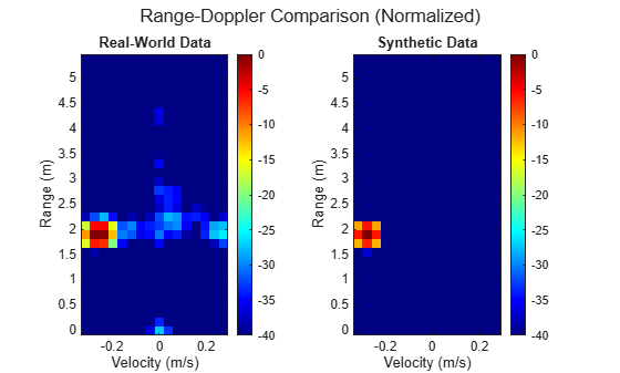
Figure contains 2 axes objects and another object of type subplottext. Axes object 1 with title Real-World Data, xlabel Velocity (m/s), ylabel Range (m) contains an object of type image. Axes object 2 with title Synthetic Data, xlabel Velocity (m/s), ylabel Range (m) contains an object of type image.

Estimate the signal-to-noise ratio (SNR) by comparing the peak response with the median level of the range-Doppler map.

syntheticSNR = max(pow2db(rgdpSynthetic(:) + eps)) - median(pow2db(rgdpSynthetic(:) + eps))

syntheticSNR = 
70.6452

realWorldSNR = max(pow2db(rgdpRealWorld(:) + eps)) - median(pow2db(rgdpRealWorld(:) + eps))

realWorldSNR = 
58.4742

Process Angle Response

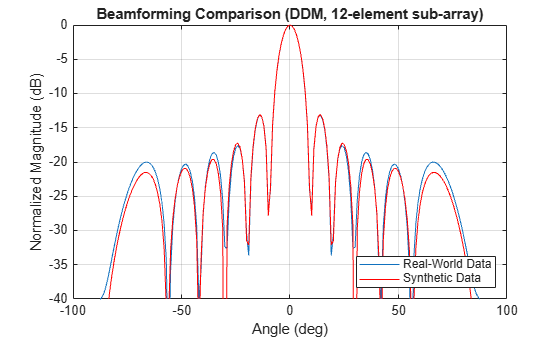
Apply the same DDM demodulation and azimuth beamforming procedure to both the synthetic and real-world datasets.

Start with the synthetic data, which contains ideal phase relationships generated by the simulation.

[~, peakSynthetic] = radarSystem.findPeaksRangeDoppler(rgdpSynthetic);
[~, bfAzSynthetic] = radarSystem.getBfAzimuthOutput(sigSynthetic, peakSynthetic);

Calibrate the Antenna Channels

The configuration file does not include antenna calibration coefficients. To compensate for hardware impairments, use the calibrateFromBoresight method to derive calibration values directly from the measured data.

For a target at boresight, the ideal steering vector has identical phase values across all channels. Any measured phase deviation therefore represents a hardware-induced error. The calibration procedure removes these phase offsets and equalizes transmit-channel amplitudes to compensate for the 1–3 dB power imbalance commonly observed across the azimuth transmitters. Without calibration, these imbalances can increase beamforming sidelobes.

Calibration requires a moving target because DDM separates transmit antenna contributions in the Doppler domain. A static target produces overlapping transmit antenna responses in the DC Doppler bin, which prevents reliable separation.

[~, peakReal] = radarSystem.findPeaksRangeDoppler(rgdpRealWorld);
movingIdx = find(abs(dpBins(peakReal(2,:))) > 0.02, 1);
peakRealMoving = peakReal(:, movingIdx);
radarSystem = radarSystem.calibrateFromBoresight(realWorldData, peakRealMoving);

After calibration, process the real-world data again and compare the beamforming response with the synthetic result.

[~, bfAzReal] = radarSystem.getBfAzimuthOutput(realWorldData, peakRealMoving);

figure;
azScanPlot = -90:90;
plot(azScanPlot, mag2db(bfAzReal(:,1)/max(bfAzReal(:,1))))
hold on;
plot(azScanPlot, mag2db(bfAzSynthetic(:,1)/max(bfAzSynthetic(:,1))), 'r')
hold off;
legend({'Real-World Data', 'Synthetic Data'}, 'Location', 'southeast')
xlabel('Angle (deg)')
ylabel('Normalized Magnitude (dB)')
title('Beamforming Comparison (DDM, 12-element sub-array)')
axis padded
ylim([-40 0])
grid on;

Figure contains an axes object. The axes object with title Beamforming Comparison (DDM, 12-element sub-array), xlabel Angle (deg), ylabel Normalized Magnitude (dB) contains 2 objects of type line. These objects represent Real-World Data, Synthetic Data.

Understand Modeling Assumptions and Calibration Considerations

The digital twin assumes ideal hardware characteristics, including equal transmit power, zero antenna phase offsets, free-space propagation, and no mutual coupling. Real radar hardware introduces additional effects, such as per-channel phase errors and transmit-channel amplitude imbalance. The boresight calibration procedure compensates for these impairments before beamforming.

Static clutter is removed by subtracting the slow-time mean from the recorded data. After calibration and clutter suppression, the remaining differences between synthetic and real-world data are small. These differences are primarily caused by thermal noise, quantization effects, interference, and target radar cross-section variation with aspect angle.

The detectDechirpSign method automatically identifies and compensates for differences between the simulation and hardware dechirp sign conventions.

Calibration is especially important for DDM systems because transmitter separation relies on phase-coherent Doppler-domain subband demodulation. Transmit-channel phase errors and amplitude imbalances can cause energy leakage between subbands and degrade angle estimation performance. In contrast, TDM separates transmitters in time and is less sensitive to transmitter-to-transmitter coupling effects.

The close agreement between calibrated real-world measurements and simulation results shows that the digital twin captures the underlying radar behavior while calibration compensates for practical hardware imperfections.