Compare Agents on Discrete Double-Integrator

R2026b

This example shows how to create and train frequently used agents on a discrete double-integrator environment. The training goal is to control the position of a mass in the second-order system by applying a force input. The example plots performance metrics such as the total training time and the total reward for each trained agent.

The results that the agents obtain in this environment, with the selected initial conditions and random number generator seed, do not necessarily imply that specific agents are better than others. Also, note that the training times depend on the computer and operating system you use to run the example, and on other processes running in the background. Your training times might differ substantially from the training times shown in the example.

Discrete Action Space Double-Integrator MATLAB Environment

The reinforcement learning environment for this example is a second-order double-integrator system with a gain and a discrete action space. The training goal is to control the position of a mass in the second-order system by applying a force input.

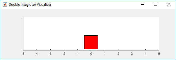
For this environment:

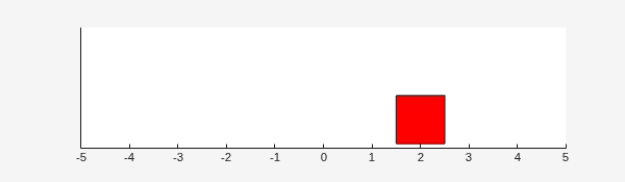
• The mass starts at an initial position of 2 m and zero velocity.

• The agent can apply one of three possible force values to the mass: -2, 0, or 2 N.

• The observations from the environment are the position and velocity of the mass.

• The episode terminates if the mass moves more than 5 m from the original position or if $\left|x\right|<0.01$.

• The reward $r_t$, which the environment provides to the agent at every time step, is a discretization of $r\left(t\right)$:

$$r\left(t\right)=-\left({x\left(t\right)}^{\prime }Qx\left(t\right)+{u\left(t\right)}^{\prime }Ru\left(t\right)\right)$$

Here:

• $x$ is the state vector of the mass.

• $u$ is the force applied to the mass.

• $Q$ is the weight on the state deviation from zero; $Q=\left[100;01\right]$.

• $R$ is the weight on the control effort; $R=0.01$.

For more information on this model, see Use Predefined Control System Environments.

Specify Random Number Stream Seed and Algorithm for Reproducibility

The example code might involve computation of random numbers at several stages. Fixing the random number stream at the beginning of some sections in the example code preserves the random number sequence in the section every time you run it, which is a necessary condition to reproduce the results. For more information, see Results Reproducibility.

Specify the random number stream with seed zero and random number algorithm Mersenne Twister. For more information on controlling the seed used for random number generation, see rng.

previousRngState = rng(0,"twister");

The output previousRngState is a structure that contains information about the previous state of the stream. You will restore the state at the end of the example.

Create Environment Object

Create a predefined environment object for the double-integrator.

env = rlPredefinedEnv("DoubleIntegrator-Discrete")

env = 
  DoubleIntegratorDiscreteAction with properties:

             Gain: 1
               Ts: 0.1000
      MaxDistance: 5
    GoalThreshold: 0.0100
                Q: [2×2 double]
                R: 0.0100
         MaxForce: 2
            State: [2×1 double]

The environment reset function initializes and returns the environment state (position and velocity).

reset(env)

ans = 2×1

     2
     0

You can visualize the double-integrator system during training or simulation using the plot function.

plot(env)

Obtain the observation and action information for later use when creating agents.

obsInfo = getObservationInfo(env)

obsInfo = 
  rlNumericSpec with properties:

     LowerLimit: -Inf
     UpperLimit: Inf
           Name: "states"
    Description: "x, dx"
      Dimension: [2 1]
       DataType: "double"

actInfo = getActionInfo(env)

actInfo = 
  rlFiniteSetSpec with properties:

       Elements: [-2 0 2]
           Name: "force"
    Description: [0×0 string]
      Dimension: [1 1]
       DataType: "double"

Configure Training and Simulation Options for All Agents

Create an evaluation object to evaluate the agent ten times without exploration every 100 training episodes.

evl = rlEvaluator(NumEpisodes=10,EvaluationFrequency=100);

Create a training options object. For this example, use the following options.

• Run the training for a maximum of 5000 episodes, with each episode lasting a maximum of 200 time steps.

• Stop the training when the average reward in the evaluation episodes is greater than –40. At this point, the agent can control the position of the mass using minimal control effort.

• To have a better insight on the agent's behavior during training, plot the training progress (default option). If you want to achieve faster training times, set the Plots option to none.

trainOpts = rlTrainingOptions( ...
    MaxEpisodes=5000, ...
    MaxStepsPerEpisode=200, ...
    StopTrainingCriteria="EvaluationStatistic", ...
    StopTrainingValue=-40);

For more information on training options, see rlTrainingOptions.

To simulate the trained agent, create a simulation options object and configure it to simulate for 500 steps.

simOptions = rlSimulationOptions(MaxSteps=500);

For more information on simulation options, see rlSimulationOptions.

Create, Train, and Simulate a Q-learning Agent

The actor and critic networks are initialized randomly. To reproduce the results of this section, specify the seed and algorithm used for random number generation.

rng(0,"twister")

First, create a default rlQAgent object using the environment specification objects.

qAgent = rlQAgent(obsInfo,actInfo);

Set a lower learning rate and a lower gradient threshold to promote a smoother (though possibly slower) training.

qAgent.AgentOptions.CriticOptimizerOptions.LearnRate = 1e-3;
qAgent.AgentOptions.CriticOptimizerOptions.GradientThreshold = 1;

Train the agent, passing the agent, the environment, and the previously defined training options and evaluator objects to train. Training is a computationally intensive process that takes several minutes to complete. To save time, load a pretrained agent by setting doTraining to false. To train the agent yourself, set doTraining to true.

doTraining = false;
if doTraining
    % To avoid plotting in training, recreate the environment.
    env = rlPredefinedEnv("DoubleIntegrator-Discrete");
    % Train the agent. Record the training time.
    tic 
    qTngRes = train(qAgent,env,trainOpts,Evaluator=evl);
    qTngTime = toc;
    % Extract number of training episodes and total steps.
    qTngEps = qTngRes.EpisodeIndex(end);
    qTngSteps = sum(qTngRes.TotalAgentSteps);
    % Uncomment to save the trained agent and the training metrics.
    % save("ddiBchQAgent.mat", ...
    %    "qAgent","qTngEps","qTngSteps","qTngTime")
else
    % Load the pretrained agent and results for the example.
    load("ddiBchQAgent.mat", ...
        "qAgent","qTngEps","qTngSteps","qTngTime")
end

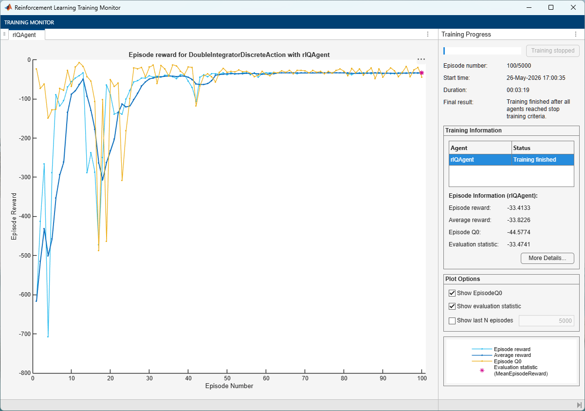
For the Q-learning agent, the training converges to a solution after 100 episodes. In the following section, check the trained agent within the double-integrator environment.

To reproduce the results of this section, specify the seed and algorithm used for random number generation.

rng(0,"twister")

Visualize the environment.

plot(env)

By default, the agent uses a greedy (hence deterministic) policy in simulation. To use the exploratory policy instead, set the UseExplorationPolicy agent property to true.

Simulate the environment with the trained agent for 500 steps and display the total reward. For more information on agent simulation, see sim.

experience = sim(env,qAgent,simOptions);

qTotalRwd = sum(experience.Reward)

qTotalRwd = 
-33.4133

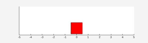
The trained Q-learning agent stabilizes the mass at the origin.

Create, Train, and Simulate a SARSA Agent

The actor and critic networks are initialized randomly. To reproduce the results of this section, specify the seed and algorithm used for random number generation.

rng(0,"twister")

First, create a default rlSARSAAgentOptions object using the environment specification objects.

sarsaAgent = rlSARSAAgent(obsInfo,actInfo);

Set a lower learning rate and a lower gradient threshold to promote a smoother (though possibly slower) training.

sarsaAgent.AgentOptions.CriticOptimizerOptions.LearnRate = 1e-3;
sarsaAgent.AgentOptions.CriticOptimizerOptions.GradientThreshold = 1;

Train the agent, passing the agent, the environment, and the previously defined training options and evaluator objects to train. Training is a computationally intensive process that takes several minutes to complete. To save time, load a pretrained agent by setting doTraining to false. To train the agent yourself, set doTraining to true.

doTraining = false;
if doTraining
    % To avoid plotting in training, recreate the environment.
    env = rlPredefinedEnv("DoubleIntegrator-Discrete");
    % Train the agent. Record the training time.
    tic 
    sarsaTngRes = train(sarsaAgent,env,trainOpts,Evaluator=evl);
    sarsaTngTime = toc;
    % Extract number of training episodes and total steps.
    sarsaTngEps = sarsaTngRes.EpisodeIndex(end);
    sarsaTngSteps = sum(sarsaTngRes.TotalAgentSteps);
    % Uncomment to save the trained agent and the training metrics.
    % save("ddiBchSARSAAgent.mat", ...
    %    "sarsaAgent","sarsaTngEps","sarsaTngSteps","sarsaTngTime")
else
    % Load the pretrained agent and results for the example.
    load("ddiBchSARSAAgent.mat", ...
        "sarsaAgent","sarsaTngEps","sarsaTngSteps","sarsaTngTime")
end

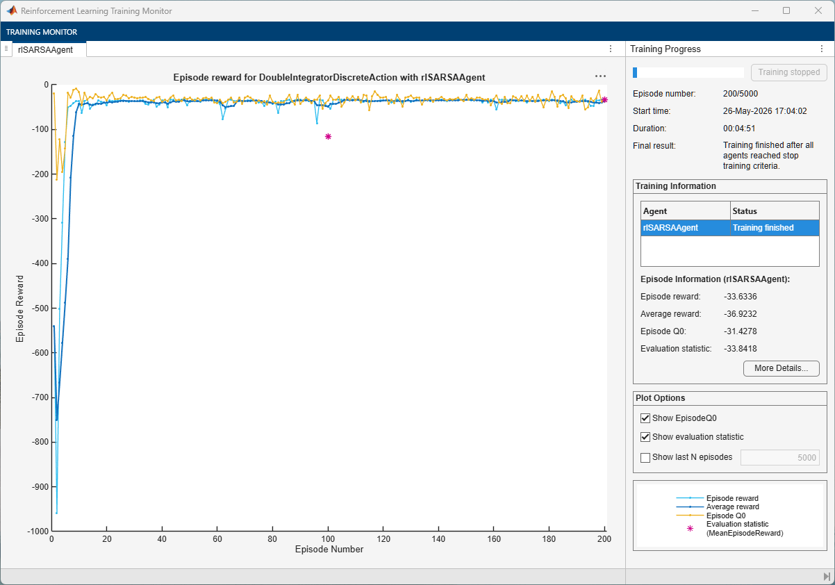
For the SARSA agent, the training converges to a solution after 200 episodes. In the following section, check the trained agent within the double-integrator environment.

To reproduce the results of this section, specify the seed and algorithm used for random number generation.

rng(0,"twister")

Visualize the environment.

plot(env)

By default, the agent uses a greedy (hence deterministic) policy in simulation. To use the exploratory policy instead, set the UseExplorationPolicy agent property to true.

Simulate the environment with the trained agent for 500 steps and display the total reward. For more information on agent simulation, see sim.

experience = sim(env,sarsaAgent,simOptions);

sarsaTotalRwd = sum(experience.Reward)

sarsaTotalRwd = 
-34.3774

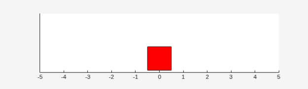
The trained SARSA agent stabilizes the mass at the origin.

Create, Train, and Simulate a DQN Agent

The actor and critic networks are initialized randomly. To reproduce the results of this section, specify the seed and algorithm used for random number generation.

rng(0,"twister")

First, create a default rlDQNAgent object using the environment specification objects.

dqnAgent = rlDQNAgent(obsInfo,actInfo);

Set a lower learning rate and a lower gradient threshold to promote a smoother (though possibly slower) training.

dqnAgent.AgentOptions.CriticOptimizerOptions.LearnRate = 1e-3;
dqnAgent.AgentOptions.CriticOptimizerOptions.GradientThreshold = 1;

Use a larger experience buffer to store more experiences, therefore decreasing the likelihood of catastrophic forgetting.

dqnAgent.AgentOptions.ExperienceBufferLength = 1e6;

Train the agent, passing the agent, the environment, and the previously defined training options and evaluator objects to train. Training is a computationally intensive process that takes several minutes to complete. To save time, load a pretrained agent by setting doTraining to false. To train the agent yourself, set doTraining to true.

doTraining = false;
if doTraining
    % To avoid plotting in training, recreate the environment.
    env = rlPredefinedEnv("DoubleIntegrator-Discrete");
    % Train the agent. Record the training time.
    tic 
    dqnTngRes = train(dqnAgent,env,trainOpts,Evaluator=evl);
    dqnTngTime = toc;
    % Extract number of training episodes and total steps.
    dqnTngEps = dqnTngRes.EpisodeIndex(end);
    dqnTngSteps = sum(dqnTngRes.TotalAgentSteps);
    % Uncomment to save the trained agent and the training metrics.
    % save("ddiBchDQNAgent.mat", ...
    %    "dqnAgent","dqnTngEps","dqnTngSteps","dqnTngTime")
else
    % Load the pretrained agent and results for the example.
    load("ddiBchDQNAgent.mat", ...
        "dqnAgent","dqnTngEps","dqnTngSteps","dqnTngTime")
end

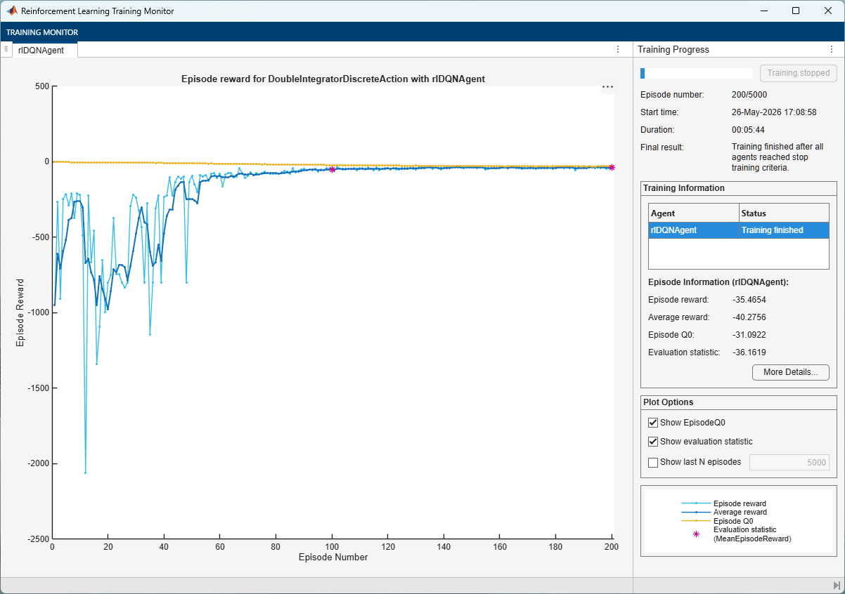
For the DQN agent, the training converges to a solution after 200 episodes. In the following section, check the trained agent within the double-integrator environment.

To reproduce the results of this section, specify the seed and algorithm used for random number generation.

rng(0,"twister")

Visualize the environment.

plot(env)

By default, the agent uses a greedy (hence deterministic) policy in simulation. To use the exploratory policy instead, set the UseExplorationPolicy agent property to true.

Simulate the environment with the trained agent for 500 steps and display the total reward. For more information on agent simulation, see sim.

experience = sim(env,dqnAgent,simOptions);

dqnTotalRwd = sum(experience.Reward)

dqnTotalRwd = 
-36.9464

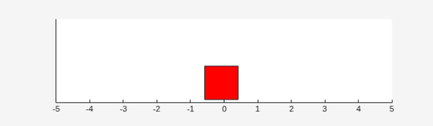
The trained DQN agent stabilizes the mass at the origin.

Create, Train, and Simulate a PG Agent

The actor and critic networks are initialized randomly. To reproduce the results of this section, specify the seed and algorithm used for random number generation.

rng(0,"twister")

First, create a default rlPGAgent object using the environment specification objects.

pgAgent = rlPGAgent(obsInfo,actInfo);

Set a lower learning rate and a lower gradient threshold to promote a smoother (though possibly slower) training.

pgAgent.AgentOptions.CriticOptimizerOptions.LearnRate = 1e-3;
pgAgent.AgentOptions.ActorOptimizerOptions.LearnRate = 1e-3;
pgAgent.AgentOptions.CriticOptimizerOptions.GradientThreshold = 1;
pgAgent.AgentOptions.ActorOptimizerOptions.GradientThreshold = 1;

Set the entropy loss weight to increase exploration.

pgAgent.AgentOptions.EntropyLossWeight = 0.005;

Train the agent, passing the agent, the environment, and the previously defined training options and evaluator objects to train. Training is a computationally intensive process that takes several minutes to complete. To save time, load a pretrained agent by setting doTraining to false. To train the agent yourself, set doTraining to true.

doTraining = false;
if doTraining
    % To avoid plotting in training, recreate the environment.
    env = rlPredefinedEnv("DoubleIntegrator-Discrete");
    % Train the agent. Record the training time.
    tic
    pgTngRes = train(pgAgent,env,trainOpts,Evaluator=evl);
    pgTngTime = toc;
    % Extract number of training episodes and total steps.
    pgTngEps = pgTngRes.EpisodeIndex(end);
    pgTngSteps = sum(pgTngRes.TotalAgentSteps);
    % Uncomment to save the trained agent and the training metrics.
    % save("ddiBchPGAgent.mat", ...
    %   "pgAgent","pgTngEps","pgTngSteps","pgTngTime")
else
    % Load the pretrained agent and results for the example.
    load("ddiBchPGAgent.mat", ...
        "pgAgent","pgTngEps","pgTngSteps","pgTngTime")
end

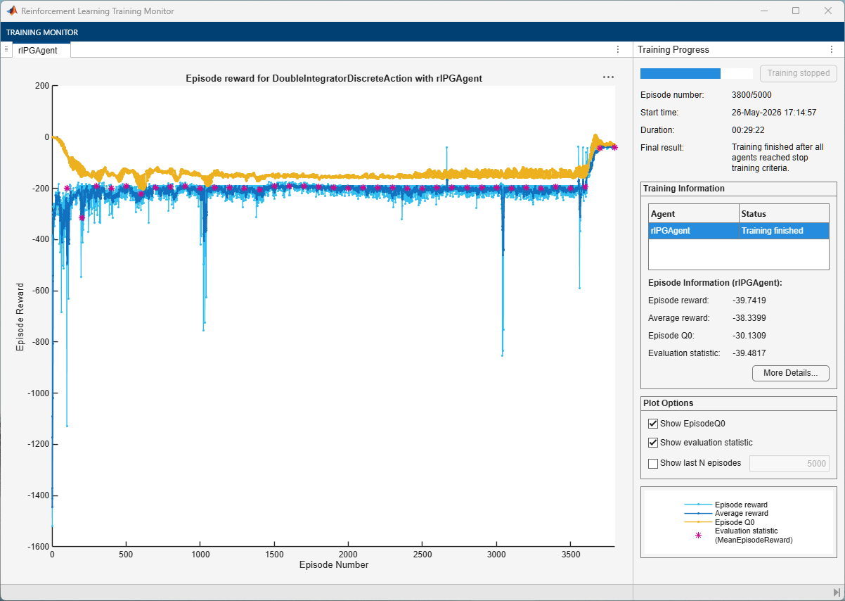
For the PG agent, the training converges to a solution after 3800 episodes. In the following section, check the trained agent within the double-integrator environment.

To reproduce the results of this section, specify the seed and algorithm used for random number generation.

rng(0,"twister")

Visualize the environment.

plot(env)

By default, the agent uses a greedy (hence deterministic) policy in simulation. To use the exploratory policy instead, set the UseExplorationPolicy agent property to true.

Simulate the environment with the trained agent for 500 steps and display the total reward. For more information on agent simulation, see sim.

experience = sim(env,pgAgent,simOptions);

pgTotalRwd = sum(experience.Reward)

pgTotalRwd = 
-48.1401

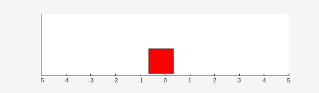
The trained PG agent stabilizes the mass at the origin with a larger error.

Create, Train, and Simulate an AC Agent

The actor and critic networks are initialized randomly. To reproduce the results of this section, specify the seed and algorithm used for random number generation.

rng(0,"twister")

First, create a default rlACAgent object using the environment specification objects.

acAgent = rlACAgent(obsInfo,actInfo);

Set a lower learning rate and a lower gradient threshold to promote a smoother (though possibly slower) training.

acAgent.AgentOptions.CriticOptimizerOptions.LearnRate = 1e-3;
acAgent.AgentOptions.ActorOptimizerOptions.LearnRate = 1e-3;
acAgent.AgentOptions.CriticOptimizerOptions.GradientThreshold = 1;
acAgent.AgentOptions.ActorOptimizerOptions.GradientThreshold = 1;

Set the entropy loss weight to increase exploration.

acAgent.AgentOptions.EntropyLossWeight = 0.005;

Train the agent, passing the agent, the environment, and the previously defined training options and evaluator objects to train. Training is a computationally intensive process that takes several minutes to complete. To save time, load a pretrained agent by setting doTraining to false. To train the agent yourself, set doTraining to true.

doTraining = false;
if doTraining
    % To avoid plotting in training, recreate the environment.
    env = rlPredefinedEnv("DoubleIntegrator-Discrete");
    % Train the agent.
    tic
    acTngRes = train(acAgent,env,trainOpts,Evaluator=evl);
    acTngTime = toc;
    % Extract number of training episodes and total steps.
    acTngEps = acTngRes.EpisodeIndex(end);
    acTngSteps = sum(acTngRes.TotalAgentSteps);
    % Uncomment to save the trained agent and the training metrics.
    % save("ddiBchACAgent.mat", ...
    %    "acAgent","acTngEps","acTngSteps","acTngTime")
else
    % Load the pretrained agent and results for the example.
    load("ddiBchACAgent.mat", ...
        "acAgent","acTngEps","acTngSteps","acTngTime")
end

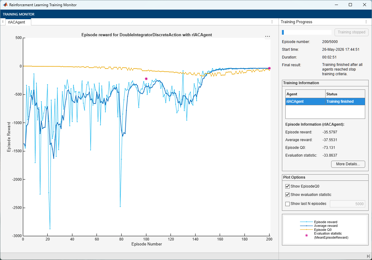
For the AC agent, the training converges to a solution after 200 episodes. In the following section, check the trained agent within the double-integrator environment.

To reproduce the results of this section, specify the seed and algorithm used for random number generation.

rng(0,"twister")

Visualize the environment.

plot(env)

By default, the agent uses a greedy (hence deterministic) policy in simulation. To use the exploratory policy instead, set the UseExplorationPolicy agent property to true.

Simulate the environment with the trained agent for 500 episodes, and display the total reward. For more information on agent simulation, see sim.

experience = sim(env,acAgent,simOptions);

acTotalRwd = sum(experience.Reward)

acTotalRwd = 
-33.4187

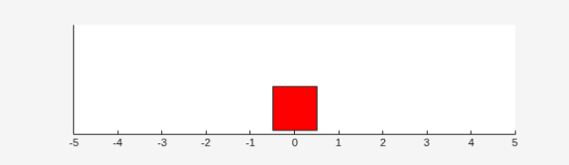
The trained AC agent stabilizes the mass at the origin.

Create, Train, and Simulate a PPO Agent

The actor and critic networks are initialized randomly. To reproduce the results of this section, specify the seed and algorithm used for random number generation.

rng(0,"twister")

First, create a default rlPPOAgent object using the environment specification objects.

ppoAgent = rlPPOAgent(obsInfo,actInfo);

Set a lower learning rate and a lower gradient threshold to promote a smoother (though possibly slower) training.

ppoAgent.AgentOptions.CriticOptimizerOptions.LearnRate = 1e-3;
ppoAgent.AgentOptions.ActorOptimizerOptions.LearnRate = 1e-3;
ppoAgent.AgentOptions.CriticOptimizerOptions.GradientThreshold = 1;
ppoAgent.AgentOptions.ActorOptimizerOptions.GradientThreshold = 1;

Train the agent, passing the agent, the environment, and the previously defined training options and evaluator objects to train. Training is a computationally intensive process that takes several minutes to complete. To save time, load a pretrained agent by setting doTraining to false. To train the agent yourself, set doTraining to true.

doTraining = false;
if doTraining
    % To avoid plotting in training, recreate the environment.
    env = rlPredefinedEnv("DoubleIntegrator-Discrete");
    % Train the agent. Record the training time.
    tic
    ppoTngRes = train(ppoAgent,env,trainOpts,Evaluator=evl);
    ppoTngTime = toc;
    % Extract number of training episodes and total steps.
    ppoTngEps = ppoTngRes.EpisodeIndex(end);
    ppoTngSteps = sum(ppoTngRes.TotalAgentSteps);
    % Uncomment to save the trained agent and the training metrics.
    % save("ddiBchPPOAgent.mat", ...
    %    "ppoAgent","ppoTngEps","ppoTngSteps","ppoTngTime")
else
    % Load the pretrained agent and results for the example.
    load("ddiBchPPOAgent.mat", ...
        "ppoAgent","ppoTngEps","ppoTngSteps","ppoTngTime")
end

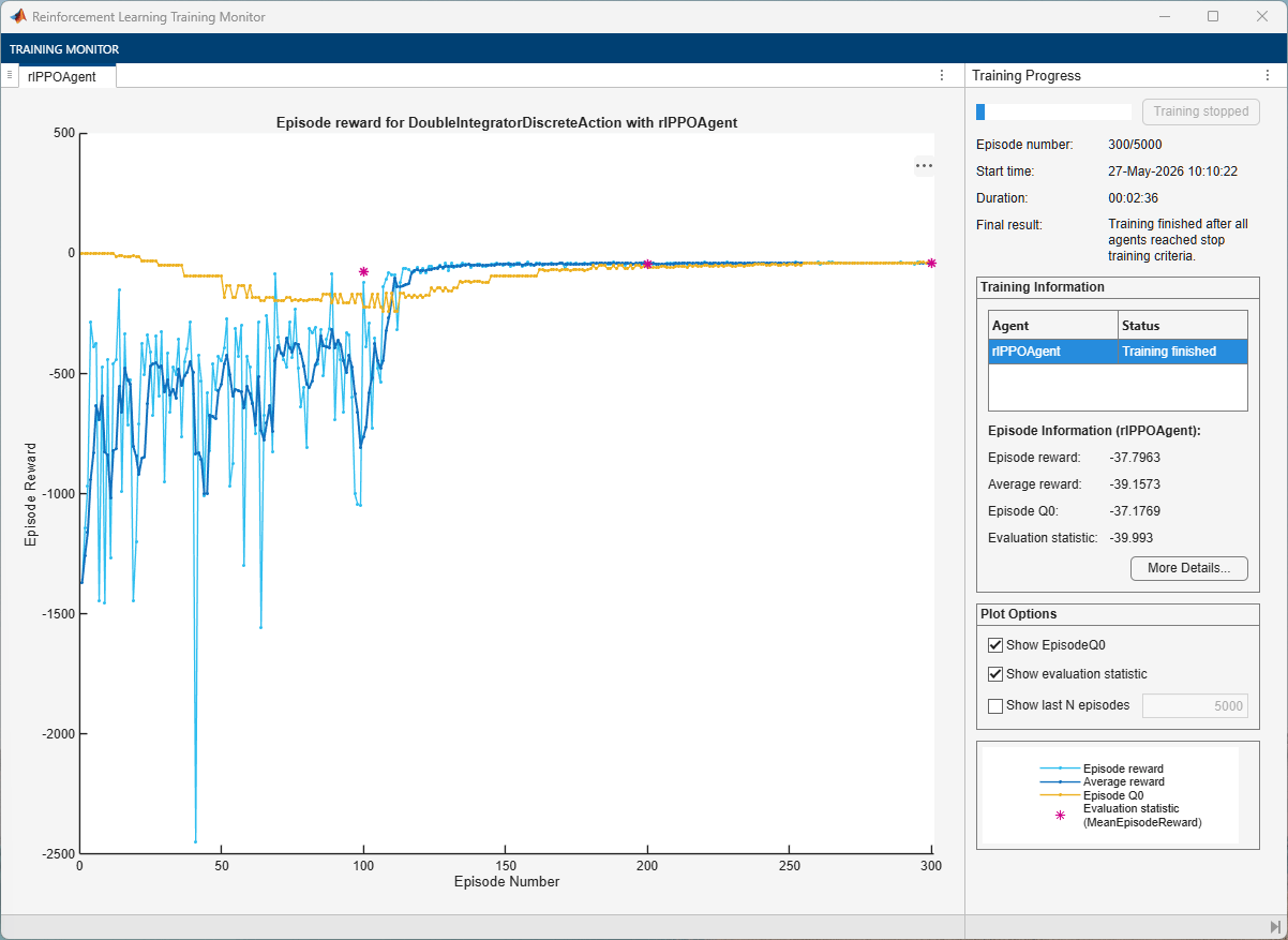
For the PPO agent, the training converges to a solution after 300 episodes. In the following section, check the trained agent within the double-integrator environment.

To reproduce the results of this section, specify the seed and algorithm used for random number generation.

rng(0,"twister")

Visualize the environment.

plot(env)

By default, the agent uses a greedy (hence deterministic) policy in simulation. To use the exploratory policy instead, set the UseExplorationPolicy agent property to true.

Simulate the environment with the trained agent for 500 steps and display the total reward. For more information on agent simulation, see sim.

experience = sim(env,ppoAgent,simOptions);

ppoTotalRwd = sum(experience.Reward)

ppoTotalRwd = 
-39.2263

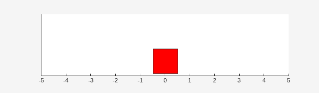
The trained PPO agent stabilizes the mass at the origin.

Create, Train, and Simulate a SAC Agent

The constructor functions initialize the agent networks randomly. To reproduce the results of this section, specify the seed and algorithm used for random number generation.

rng(0,"twister")

Create a default rlSACAgent object using the environment specification objects.

sacAgent = rlSACAgent(obsInfo,actInfo);

Set a lower learning rate and a lower gradient threshold to promote a smoother (though possibly slower) training.

sacAgent.AgentOptions.CriticOptimizerOptions(1).LearnRate = 1e-3;
sacAgent.AgentOptions.CriticOptimizerOptions(2).LearnRate = 1e-3;
sacAgent.AgentOptions.CriticOptimizerOptions(1).GradientThreshold = 1;
sacAgent.AgentOptions.CriticOptimizerOptions(2).GradientThreshold = 1;

sacAgent.AgentOptions.ActorOptimizerOptions.LearnRate = 1e-3;
sacAgent.AgentOptions.ActorOptimizerOptions.GradientThreshold = 1;

Set the initial entropy weight and target entropy to increase exploration.

sacAgent.AgentOptions.EntropyWeightOptions.EntropyWeight = 0.005;
sacAgent.AgentOptions.EntropyWeightOptions.TargetEntropy = 0.5;

Use a larger experience buffer to store more experiences, therefore decreasing the likelihood of catastrophic forgetting.

sacAgent.AgentOptions.ExperienceBufferLength = 1e6;

Train the agent, passing the agent, the environment, and the previously defined training options and evaluator objects to train. Training is a computationally intensive process that takes several minutes to complete. To save time, load a pretrained agent by setting doTraining to false. To train the agent yourself, set doTraining to true.

doTraining = false;
if doTraining
    % To avoid plotting in training, recreate the environment.
    env = rlPredefinedEnv("DoubleIntegrator-Discrete");
    % Train the agent. Record the training time.
    tic
    sacTngRes = train(sacAgent,env,trainOpts,Evaluator=evl);
    sacTngTime = toc;
    % Extract number of training episodes and total steps.
    sacTngEps = sacTngRes.EpisodeIndex(end);
    sacTngSteps = sum(sacTngRes.TotalAgentSteps);
    % Uncomment to save the trained agent and the training metrics.
    % save("ddiBchSACAgent.mat", ...
    %    "sacAgent","sacTngEps","sacTngSteps","sacTngTime")
else
    % Load the pretrained agent and results for the example.
    load("ddiBchSACAgent.mat", ...
        "sacAgent","sacTngEps","sacTngSteps","sacTngTime")
end

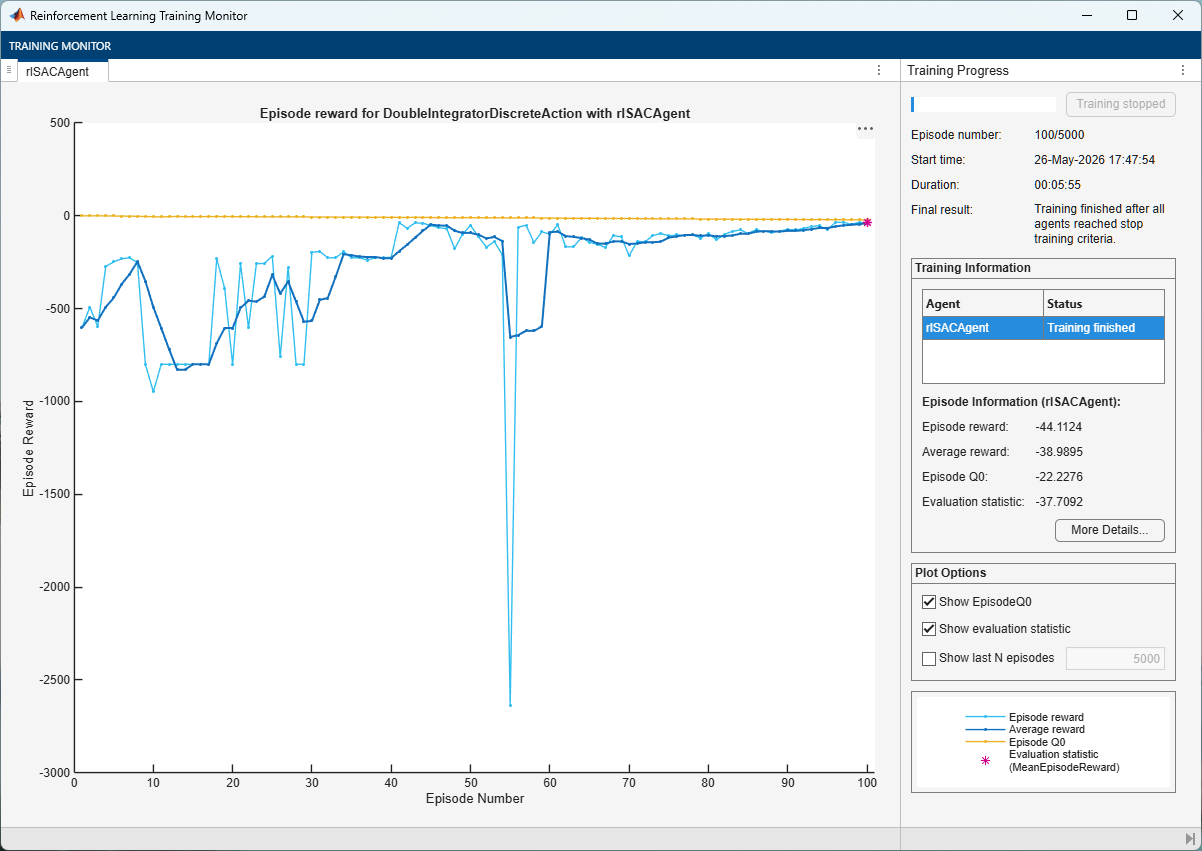
For the SAC agent, the training converges to a solution after 200 episodes. In the following section, check the trained agent within the cart-pole environment.

To reproduce the results of this section, specify the seed and algorithm used for random number generation.

rng(0,"twister")

Visualize the environment.

plot(env)

By default, the agent uses a greedy (hence deterministic) policy in simulation. To use the exploratory policy instead, set the UseExplorationPolicy agent property to true.

Simulate the environment with the trained agent for 500 steps. For more information on agent simulation, see rlSimulationOptions and sim.

simOptions = rlSimulationOptions(MaxSteps=500);
experience = sim(env,sacAgent,simOptions);

sacTotalRwd = sum(experience.Reward)

sacTotalRwd = 
-49.4178

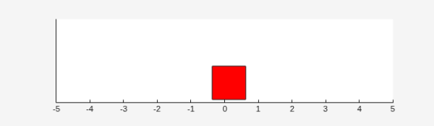
The trained SAC agent stabilizes the mass at the origin.

Plot Training and Simulation Metrics

For each agent, collect the total reward from the final simulation episode, the number of training episodes, the total number of agent steps, and the total training time as shown in the Reinforcement Learning Training Monitor. Because the PG agent training takes much longer to converge to a solution, do not include the PG agent data.

simReward = [
    qTotalRwd
    sarsaTotalRwd
    dqnTotalRwd
    acTotalRwd
    ppoTotalRwd
    sacTotalRwd
    ];

tngEpisodes = [
    qTngEps
    sarsaTngEps
    dqnTngEps
    acTngEps
    ppoTngEps
    sacTngEps
    ];

tngSteps = [
    qTngSteps
    sarsaTngSteps
    dqnTngSteps
    acTngSteps
    ppoTngSteps
    sacTngSteps
    ];

tngTime = [
    dqnTngTime
    qTngTime
    sarsaTngTime
    acTngTime
    ppoTngTime
    sacTngTime
    ];

Plot the simulation reward, number of training episodes, number of training steps (that is, the number of interactions between the agent and the environment) and the training time. Scale the data by the factor [30 200 2e6 600] for better visualization.

bar([simReward,tngEpisodes,tngSteps,tngTime]./[30 200 2e6 600])
xticklabels(["Q" "SARSA" "DQN" "AC" "PPO" "SAC"])
legend( ...
    "Total Reward","Training Episodes", ...
    "Training Steps","Training Time", ...
    "Location","northeast")

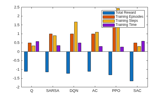
The plot shows that, for this environment, and with the used random number generator seed and initial conditions, PPO and AC have the lowest training time, despite needing more steps and episodes to converge. By contrast, SAC (due to its more complex algorithm that needs to calculate more gradients), uses less episodes and steps but more training time. The differences in cumulative reward over a simulation episode are minimal, with Q-learning, SARSA and AC performing slightly better than the other agents. With a different random seed, the initial agent networks would be different, and therefore, convergence results might be different. For more information on the relative strengths and weaknesses of each agent, see Reinforcement Learning Agents.

Save all the variables created in this example, including the training results, for later use.

% Uncomment the following line to save all the workspace variables
% save ddiAllVariables.mat

Restore the random number stream using the information stored in previousRngState.

rng(previousRngState);