Resample Nonuniformly Sampled Signals
This example shows how to resample nonuniformly sampled signals to a new uniform rate. It shows how to apply a custom filter on irregularly sampled data to reduce aliasing. It also shows how to use detrending to remove transients at the start and at the end of the signal.
Resampling Nonuniformly Sampled Signals to a Desired Rate
The resample function allows you to convert a nonuniformly sampled signal to a new uniform rate.
Create a 500 Hz sinusoid sampled irregularly at about 48 kHz. We simulate the irregularity by adding random values to the uniform vector.
rng("default")
nominalFs = 48000;
f = 500;
Tx = 0:1/nominalFs:0.01;
irregTx = sort(Tx + 1e-4*rand(size(Tx)));
x = sin(2*pi*f*irregTx);
plot(irregTx,x,".")

To resample a nonuniformly sampled signal, you can call resample with a time vector input.
The next example converts our original signal to a uniform 44.1 kHz rate.
desiredFs = 44100;
[y, Ty] = resample(x,irregTx,desiredFs);
plot(irregTx,x,".-",Ty,y,"o-")
legend("Original","Resampled")
ylim([-1.2 1.2])
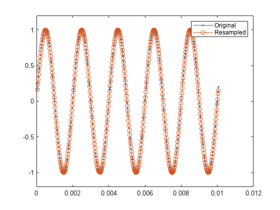
You can see that our resampled signal has the same shape and size as the original signal.
Choosing an Interpolation Method
The conversion algorithm in resample works best when the input samples are as close to regularly spaced as possible, so it is instructive to observe what may happen when a section of the input samples is missing from the sampled data.
The next example notches out the second crest of the input sinusoid and apply resampling.
irregTx(105:130) = [];
x = sin(2*pi*f*irregTx);
[y, Ty] = resample(x,irregTx,desiredFs);

plot(irregTx,x,". ")
hold on
plot(Ty,y,".-")
hold off
legend("Original","Resampled")
ylim([-1.2 1.2])

The missing segment is connected by linear interpolation. Linear interpolation is the default method used by the resample function to resample nonuniformly sampled data.
In some cases where you have missing data or large gaps in your input, you can recover some of the missing data by choosing a different interpolation method.
For low-noise, low-bandwidth signals, splines can be very effective when used to reconstruct the original signal. To use a cubic spline during resampling, supply the "spline" interpolation method:
[y, Ty] = resample(x,irregTx,desiredFs,"spline");

plot(irregTx,x,". ")
hold on
plot(Ty,y,".-")
hold off
legend("Original","Resampled using ""spline""")
ylim([-1.2 1.2])

Controlling the Interpolation Grid
By default, resample constructs an intermediate grid that is a close rational approximation of the ratio between the desired sample rate and the average sample rate of the signal.
If a section of your input samples contain high-frequency components, you can control the spacing of the intermediate grid by choosing integer coefficients, p and q, to select this rational ratio.
Examine the step response of an underdampened second order filter that oscillates at a rate of about 3 Hz:
w = 2*pi*3;
d = .1002;
z = sin(d);
a = cos(d);

t = [0:0.05:2 3:8];

x = 1 - exp(-z*w*t).*cos(w*a*t-d)/a;
plot(t,x,".-")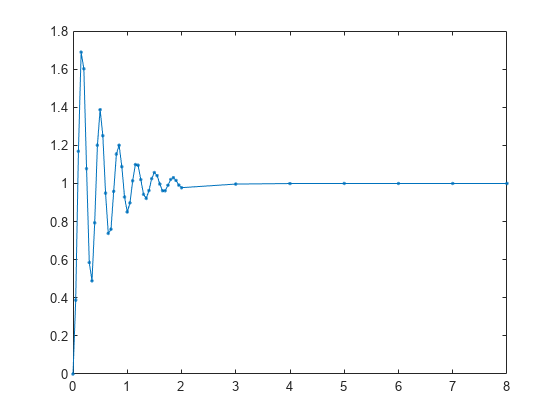
The step response is sampled at a high rate where it is oscillating and at a low rate where it is not.
Now resample the signal at 100 Hz just using the default settings:
Fs = 100;
[y, Ty] = resample(x,t,Fs);
plot(t,x,". ")
hold on
plot(Ty,y)
hold off
legend("Original","Resampled (default settings)")
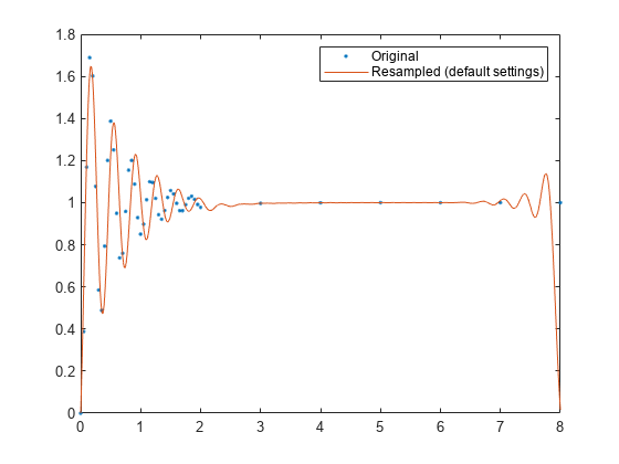
The envelope of the oscillation at the start of the waveform is attenuated and oscillates more slowly than the original signal.
resample, by default, interpolates to a grid of regularly spaced intervals that correspond to the average sample rate of the input signal.
avgFs = (numel(t)-1) /(t(end)-t(1))
avgFs =
5.7500
The sample rate of the grid should be higher than twice the largest frequency that you want to measure. The sample rate of the grid, 5.75 samples per second, is below the Nyquist sample rate, 6 Hz, of the ringing frequency.
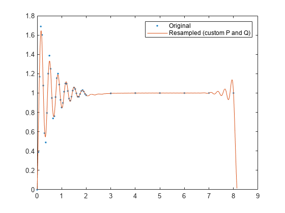
To make the grid have a higher sample rate, you can supply the integer parameters, p and q. resample adjusts the sample rate of the grid to Q*Fs/P, interpolates the signal, and then applies its internal sample rate converter (upsampling by P and downsampling by Q) to recover the desired sample rate, Fs. Use rat to select p and q.
Since the ringing of the oscillation is 3 Hz, specify the grid with a sample rate of 7 Hz, which is a little higher than the Nyquist rate. The headroom of 1 Hz accounts for additional frequency content due to the decaying exponential envelope.
Fgrid = 7;
[p,q] = rat(Fs/Fgrid)
p =
100
q =
7
[y, Ty] = resample(x,t,Fs,p,q);
plot(t,x,".")
hold on
plot(Ty,y)
hold off
legend("Original","Resampled (custom P and Q)")
Specifying the Anti-Aliasing Filter
In the next example, you can view the output of a digitizer that measures the throttle setting on an airplane engine. The throttle setting is nonuniformly sampled about a nominal rate of 100 Hz. We will try to resample this signal at a uniform 10 Hz rate.
Here are the samples of our original signal.
load engineRPM
plot(t,x,".")
xlabel("Time (s)")
ylabel("RPM")
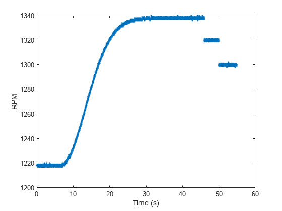
Our signal is quantized. Now zoom into the ascending region in the time interval from 20 seconds to 23 seconds:
plot(t,x,".")
xlim([20 23])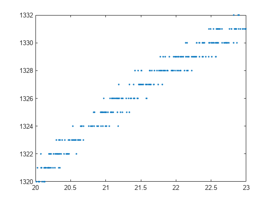
The signal is slowly varying within this region. This allows you to remove some of the quantization noise by using the anti-aliasing filter in the resampler.
desiredFs = 10;
[y,ty] = resample(x,t,desiredFs);

plot(t,x,".")
hold on
plot(ty,y,".-")
hold off
xlabel("Time")
ylabel("RPM")
legend("Original","Resampled")
xlim([20 23])

This works reasonably well. However, the resampled signal can be smoothed further by providing resample a filter with a low cutoff frequency.
First, set the grid spacing to be about our nominal 100 Hz sample rate.
nominalFs = 100;
Next, determine a reasonable p and q to obtain the desired rate. Since the nominal rate is 100 Hz and our desired rate is 10 Hz, you need to decimate by 10. This is equivalent to setting p to 1 and setting q to 10.
p = 1;
q = 10;
You can supply resample with your own filter. To have proper temporal alignment, the filter should be of odd length. The filter length should be a few times larger than p or q (whichever is larger). Set the cutoff frequency to be 1 / q desired cutoff and then multiply the resulting coefficients by p.
% ensure an odd length filter
n = 10*q+1;

% use .25 of Nyquist range of desired sample rate
cutoffRatio = .25;

% construct lowpass filter
lpFilt = p * fir1(n, cutoffRatio * 1/q);

% resample and plot the response
[y,ty] = resample(x,t,desiredFs,p,q,lpFilt);

plot(t,x,".")
hold on
plot(ty,y)
hold off
xlabel("time")
ylabel("RPM")
legend("Original","Resampled (custom filter)",Location="best")
xlim([20 23])

Removing Endpoint Effects
Now zoom out to view our original signal. Note that there is significant offset at the endpoints.
plot(t,x,".",ty,y)
xlabel("time")
ylabel("RPM")
legend("original","resampled (custom filter)",Location="best")
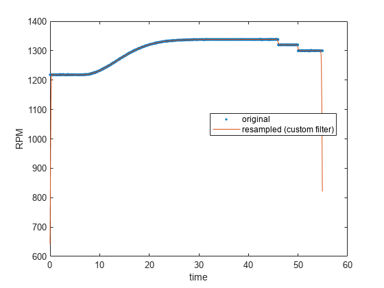
These artifacts arise because resample assumes that the signal is zero outside the borders of the signal. To reduce the effect of these discontinuities, subtract off a line between the endpoints of the signal, perform resampling, and then add back the line to the original function. You can do this by computing the slope and the offset of the line between the first and last sample, and using polyval to construct the line to subtract.
% compute slope and offset (y = a1 x + a2)
a(1) = (x(end)-x(1)) / (t(end)-t(1));
a(2) = x(1);

% detrend the signal
xdetrend = x - polyval(a,t);
plot(t,xdetrend)

The detrended signal now has both of its endpoints near zero, which reduces the transients introduced. Call resample and then add back the trend.
[ydetrend,ty] = resample(xdetrend,t,desiredFs,p,q,lpFilt);

y = ydetrend + polyval(a,ty);

plot(t,x,".",ty,y)
xlabel("Time")
ylabel("RPM")
legend("Original","Resampled (detrended, custom filter)", ...
    Location="best")

Summary
This example shows how to use resample to convert uniformly and nonuniformly sampled signals to a fixed rate.
Further Reading
For more information on reconstructing nonuniformly spaced samples with custom splines, you can consult the Curve Fitting Toolbox™ documentation.