Optimize Liquid Cooling System of Inverter

R2026b

This example shows how to analyze the performance of a liquid cooling system for a three-phase inverter. To find the steady-state temperatures and losses, you first run detailed and reduced order models (ROM). Then you compute the optimal size of the heatsink that maximizes the inverter efficiency and minimizes the lifetime cost.

Model Overview

Open the model sscv_inverter_liquid_cooling.

model = 'sscv_inverter_liquid_cooling';
open_system(model)
sscv_inverter_liquid_cooling_params;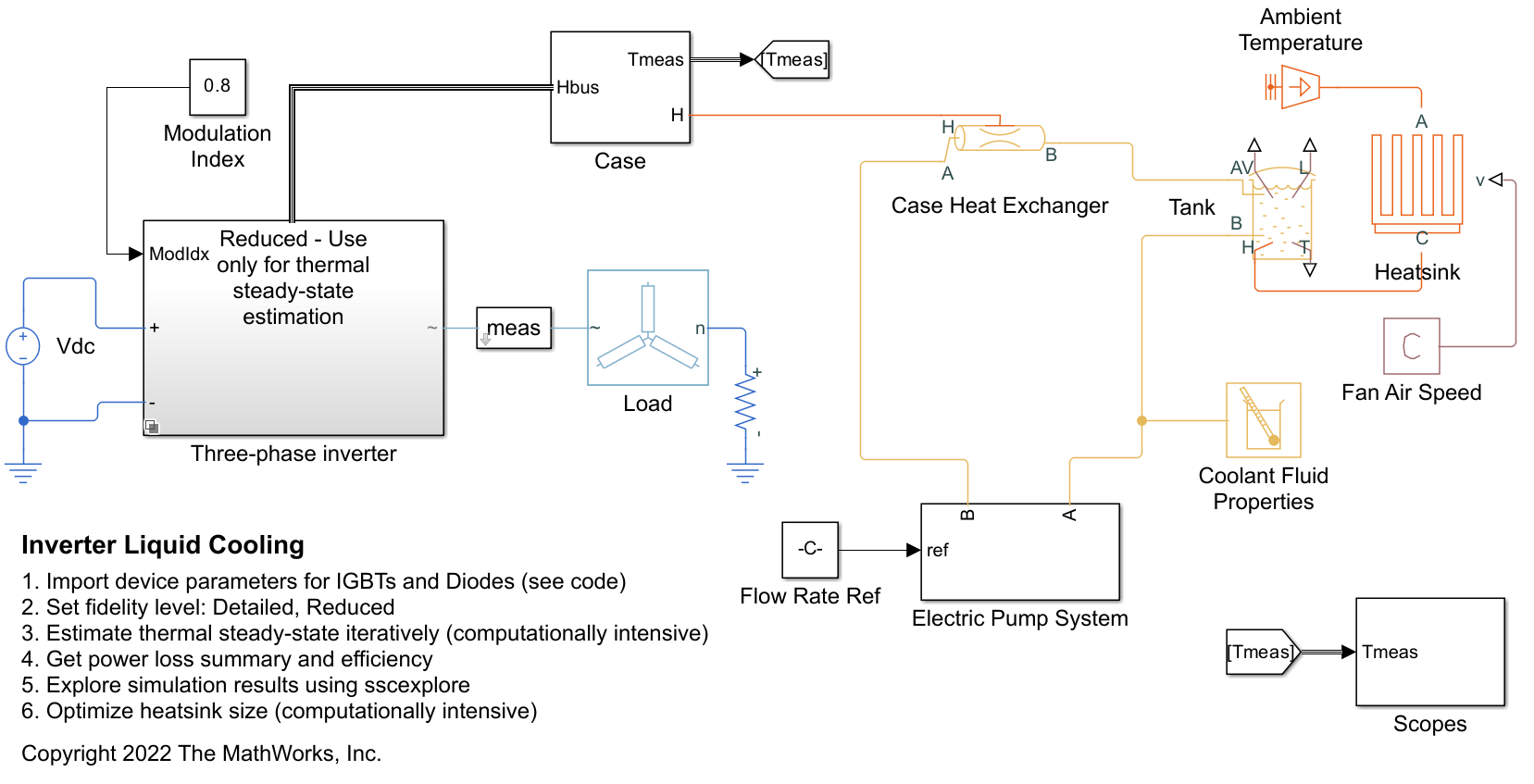

To drive the Load block, the inverter converts the DC power from the high-voltage battery into three-phase AC power. Conduction losses, switching losses, and reverse recovery losses generate heat in the case. Liquid cooling is effective to dissipate heat in the order of kilowatts. Liquid coolant flows in the inverter case to exchange heat. The Electric Pump System provides the hydraulic power to produce the flow. Then, the hot liquid flows into a heatsink to dissipate the heat. The heatsink is also called radiator. Fans blow air into the radiator to increase heat dissipation via forced convection.

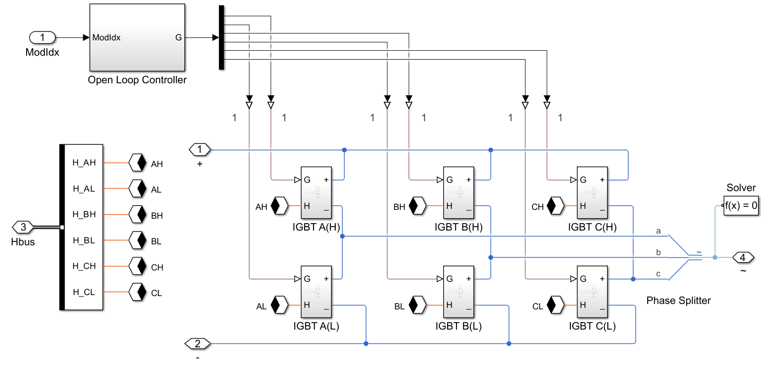
The Three-Phase Inverter subsystem has a Detailed Inverter variant that comprises six IGBT switching devices and their body diodes.

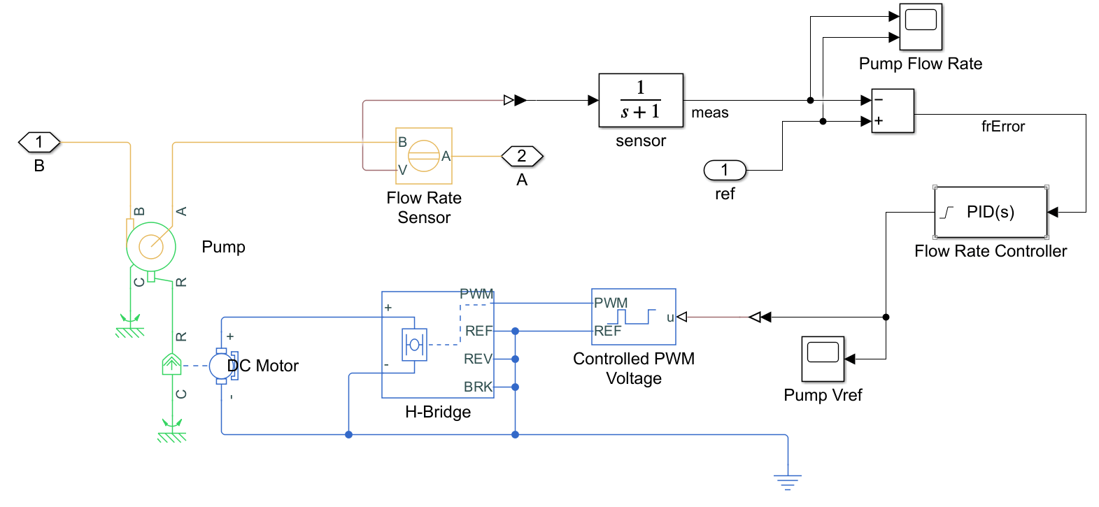
The subsystem of Electric Pump System comprises a 12V DC motor, a H-bridge driver, and a small centrifugal pump. The motor regulates the pump flow rate by using PWM switching and a PID controller:

Import Device Parameters

In the Detailed Inverter variant, to import the datasheet parameters for the IGBTs and the integral diodes, including the turn-on and turn-off switching losses for the IGBT blocks, and the reverse recovery losses for the Diode blocks, use the ee_importDeviceParameters function.

sscv_inverter_liquid_cooling_import

The plots above show the device characteristics for the imported IGBT and Diode blocks, including switching and reverse recovery losses.

Run a Detailed Simulation

Simulate 4 AC cycles to observe load voltage and current.

set_param([model, '/Three-Phase Inverter'],'LabelModeActiveChoice', 'Detailed')
stopTime = 4/60; %#ok<NASGU> 
out = sim(model);
figure();
Vabc = out.simlog.Load.N.V.series;
Iabc = out.simlog.Load.wye_impedance.I.series;
subplot(2,1,1);
plot(Vabc.time, Vabc.values('V'));
ylabel('Phase voltages [V]')
grid on
subplot(2,1,2);
plot(Iabc.time, Iabc.values('A'));
xlabel('Time [s]')
ylabel('Phase currents [A]')
grid on

Observe the inverter successfully produces a three-phase current at 60 Hz. It achieves electrical AC steady-state after an initial transient cycle.

Run a Reduced Thermal Simulation

The electrical characteristic times in the inverter subsystem are in the order of milliseconds, but the thermal characteristic times are in the order of minutes. If you are only interested in the thermal steady-state of the system for a particular cooling setup and a fixed value of average conduction and switching losses, you can use the Reduced - Use only for thermal steady-state estimation variant of the Three-phase inverter subsystem.

To run a 1 hour simulation of thermal model with constant conduction and switching losses, but without voltages or currents, at the MATLAB Command Window, enter:

set_param([bdroot, '/Three-Phase Inverter'],'LabelModeActiveChoice', 'Reduced - Use only for thermal steady-state estimation');
stopTime = 3600;
out = sim(model);

Plot the temperature of the case, heatsink, and coolant parts:

figure();
Tcase = out.simlog.Case_Heat_Exchanger.H.T.series;
Theatsink = out.simlog.Heatsink.T_hs.series;
Tcoolant = out.simlog.Tank.T_I.series;
hold on
plot(Tcase.time, Tcase.values('degC'));
plot(Theatsink.time, Theatsink.values('degC'));
plot(Tcoolant.time, Tcoolant.values('degC'));
hold off
grid on
legend({'Case', 'Heatsink', 'Coolant'})
xlabel('Time [s]')
ylabel('Temperature [degC]')

You observe that it takes almost one hour to reach thermal steady state.

Estimate Thermal Steady-State Iteratively

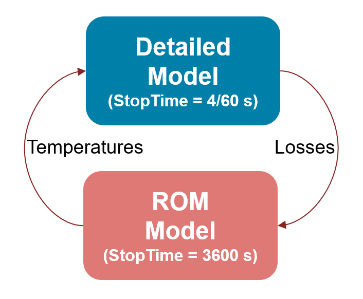
To find the accurate steady-state losses and temperatures faster, first compute the accurate losses at a given temperature by using the Detailed Inverter option of the Three-Phase Inverter subsystem. Then compute the accurate steady-state temperatures at a given loss by using the Reduced option of the Three-Phase Inverter subsystem.

Finally, iterate between these two processes to estimate the thermal steady-state.

sscv_inverter_liquid_cooling_thermal_ss

You observe that 3 iterations are enough to find a thermal steady-state with a reasonable accuracy of +-2 degC.

Optimize Heatsink Size for Cost and Efficiency

To find the best option that minimizes the cost and maximizes the efficiency, repeat the steady-state iterations for several heatsink sizes. At the MATLAB Command Window, enter:

displayOutputs = false;
sscv_inverter_liquid_cooling_optimize

You observe that the option with a good blend of high efficiency and low coolant temperature, with a minimum lifetime cost, is a heatsink with around 120 fins.