Read Data from BLF Files Using ARXML

This example shows you how to read data from a BLF file using ARXML as the database.

Open the ARXML File

Open the ARXML file DecodingExample.arxml using arxmlDatabase function.

arxmlObj = arxmlDatabase("DecodingExample.arxml")

arxmlObj = 
  Database with properties:

    Name: "DecodingExample.arxml"
    Path: "C:\ExampleManager772791\user.Example_ARXMLCANDecoding\vnt-ex11728030\DecodingExample.arxml"
     CAN: [1×1 shared.vnt.arxml.protocol.CAN]

View Details of the BLF File

Retrieve and view information about the BLF file. The blfinfo function parses general information about the format and contents of the Vector Binary Logging Format (BLF) file and returns the information as a structure.

blfin = blfinfo("BLF_ARXML.blf")

blfin = struct with fields:
                  Name: "BLF_ARXML.blf"
                  Path: "C:\ExampleManager772791\user.Example_ARXMLCANDecoding\vnt-ex11728030\BLF_ARXML.blf"
           Application: "CANoe"
    ApplicationVersion: "18.2.65"
               Objects: 6075
             StartTime: 15-Nov-2024 18:06:16.345
               EndTime: 15-Nov-2024 18:07:17.460
           ChannelList: [2×3 table]

blfin.ChannelList

ans=2×3 table
    1    "CAN"    6070
    2    "CAN"       0

Read Data from the BLF File

The data of interest was stored in channel 1 of the BLF file. Read the CAN data using the blfread function. You can also provide the ARXML file to the function call to enable message name lookup and signal value decoding.

blfData = blfread("BLF_ARXML.blf", 1, "Database", arxmlObj)

blfData=6070×8 timetable
    0.050294 sec         2048    1    'Frame2'                [250,0,16,0,4,0,1,0]    8    1×1 struct    0    0
    0.050526 sec            3    0    'Frame4'    [210,236,104,118,52,187,124,192]    8    1×1 struct    0    0
    0.050694 sec           16    0    'Frame5'                        [0,3,89,100]    4    1×1 struct    0    0
    0.050898 sec         2047    0    'Frame1'             [226,99,235,64,255,255]    6    1×1 struct    0    0
    0.051184 sec    536870911    1    'Frame3'           [0,0,45,10,68,26,184,161]    8    1×1 struct    0    0
     0.10029 sec         2048    1    'Frame2'                [237,0,12,0,6,0,0,0]    8    1×1 struct    0    0
     0.10053 sec            3    0    'Frame4'          [0,56,252,27,254,13,75,64]    8    1×1 struct    0    0
     0.10071 sec           16    0    'Frame5'                      [0,252,200,92]    4    1×1 struct    0    0
     0.10091 sec         2047    0    'Frame1'               [68,41,41,64,249,255]    6    1×1 struct    0    0
      0.1012 sec    536870911    1    'Frame3'          [0,64,126,0,196,46,248,98]    8    1×1 struct    0    0
     0.15029 sec         2048    1    'Frame2'                [118,0,24,0,4,0,0,0]    8    1×1 struct    0    0
     0.15052 sec            3    0    'Frame4'        [120,21,188,10,94,69,132,64]    8    1×1 struct    0    0
     0.15069 sec           16    0    'Frame5'                      [0,252,161,14]    4    1×1 struct    0    0
     0.15089 sec         2047    0    'Frame1'              [41,48,20,192,254,255]    6    1×1 struct    0    0
      ⋮

View the signals of interest included in the Frame2 message.

blfData.Signals{1}

ans = struct with fields:
     Signal5: 27
    Signal11: 7

Repackage and Visualize Signal Values of Interest

Use the canSignalTimetable function to repackage signal data from each unique message on the bus into a signal timetable.

signalTimetable = canSignalTimetable(blfData, "Frame2")

signalTimetable=1214×2 timetable
    0.050294 sec         27         7
     0.10029 sec    20.5000    6.5000
     0.15029 sec         89         8
     0.20029 sec        -22         8
     0.25029 sec         68         7
     0.30029 sec    10.5000         7
     0.35029 sec        -19    7.5000
     0.40029 sec         13         6
      0.4503 sec    40.5000    5.5000
     0.50029 sec    51.5000    6.5000
     0.55029 sec         -4    6.5000
     0.60029 sec         -8    6.5000
     0.65029 sec        -14    5.5000
     0.70029 sec        -28    6.5000
      ⋮

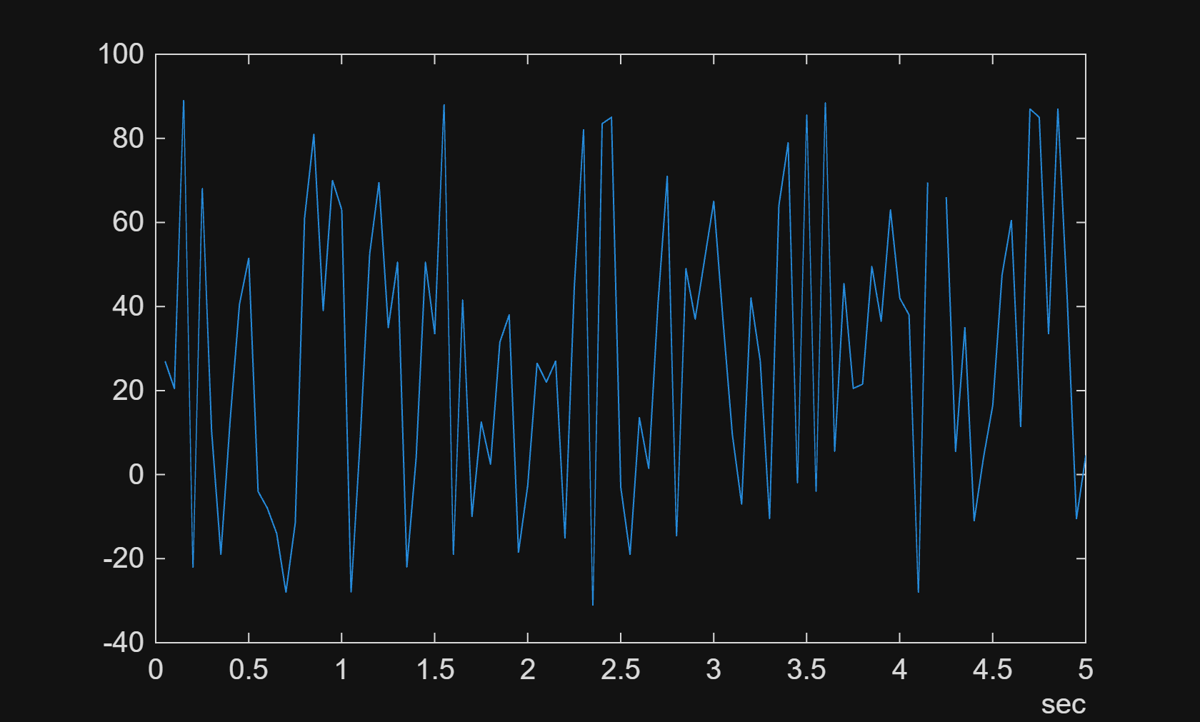
To visualize the signals of interest, columns from the signal timetables can be plotted over time for further analysis. The plot shows the first 5 seconds value for the Signal5.

plot(signalTimetable.Time, signalTimetable.Signal5); 
xlim(seconds([0 5]));