5G NR Waveform Acquisition and Analysis
This example shows how to generate a 5G NR test model (NR-TM) waveform using the 5G Waveform Generator app and download the generated waveform to a Keysight™ vector signal generator for over-the-air transmission using the Instrument Control Toolbox™ software. The example then captures the transmitted over-the-air signal using a Keysight signal analyzer and analyzes the signal in MATLAB®.
Introduction
This example generates a 5G NR-TM waveform using the 5G Waveform Generator app, downloads and transmits the waveform onto a Keysight vector signal generator, and then receives the waveform using a Keysight signal analyzer for waveform analysis in MATLAB. This diagram shows the general workflow.

Requirements
To run this example, you need these instruments:
Keysight E4438C ESG vector signal generator
Keysight N9030A PXA signal analyzer
Generate Baseband Waveform Using 5G Waveform Generator App
In MATLAB, on the Apps tab, click the 5G Waveform Generator app.
In the Waveform Type section, click NR Test Models. In the left-most pane of the app, you can set the parameters for the selected waveform. For this example:
Set Frequency range as
FR1 (410 MHz - 7.125 GHz)Set Test model as
NR-FR1-TM3.1 (Full band, uniform 64 QAM)Set Channel bandwidth (MHz) as
10Set Subcarrier spacing (kHz) as
30Set Duplex mode as
FDDSet Subframes as
10
On the app toolstrip, click Generate.
% Set the NR-TM parameters for the receiver
nrtm = "NR-FR1-TM3.1"; % Reference channel
bw   = "10MHz";        % Channel bandwidth
scs  = "30kHz";        % Subcarrier spacing
dm   = "FDD";          % Duplexing mode
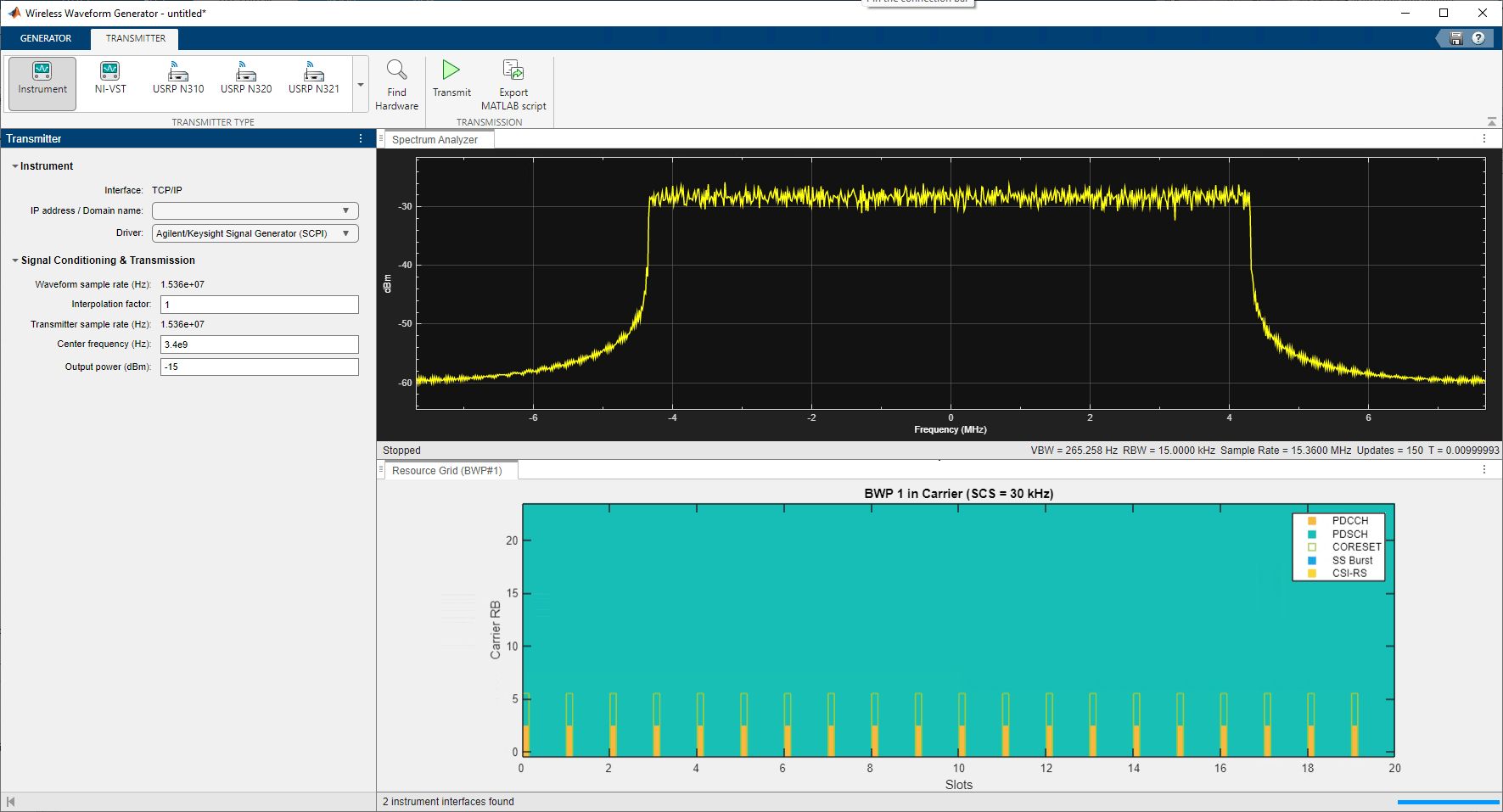
This figure shows a 10 MHz 5G NR waveform visible at baseband.

Transmit Over-the-Air Signal
Download the generated signal to the RF signal generator over one of the supported communication interfaces (requires Instrument Control Toolbox). The app automatically finds the signal generator that is connected over the TCP/IP interface. On the Transmitter tab of the app, select Agilent/Keysight Signal Generator SCPI from the Driver list. Set the Center frequency (Hz) parameter to 3.4e9 and the Output power (dBm) parameter to -15. The app automatically obtains the baseband sample rate from the generated waveform. To start the transmission, click Transmit in the toolstrip.
Read IQ Data from a Signal Analyzer over TCP/IP
To read the in-phase and quadrature (IQ) data into MATLAB for analysis, configure the Keysight N9030A signal analyzer using the Instrument Control Toolbox software.
Define the instrument configuration parameters based on the signal you are measuring.
% Set parameters for the spectrum analyzer
centerFrequency = 3.4e9;
sampleRate = 15.36e6;
measurementTime = 20e-3;
mechanicalAttenuation = 0; %dB
startFrequency = 3.39e9;
stopFrequency = 3.41e9;
resolutionBandwidth = 220e3;
videoBandwidth = 220000;
Perform these steps before connecting to the spectrum analyzer.
Find the resource ID of the Keysight N9030A signal analyzer.
Connect to the instrument using the virtual instrument software architecture (VISA) interface.
Adjust the input buffer size to hold the data that the instrument returns.
Set the timeout to allow sufficient time for the measurement and data transfer.
foundVISA = visadevlist;
resourceID = foundVISA(foundVISA.Model == "N9030A",:).ResourceName;
resourceID = resourceID(contains(resourceID,"N9030A"));             % Extract resourceID which contains "N9030A"
sigAnalyzerObj = visadev(resourceID);
sigAnalyzerObj.ByteOrder = "big-endian";
sigAnalyzerObj.Timeout = 20;
Reset the instrument to a known state using the appropriate standard command for programmable instruments (SCPI). Query the instrument identity to ensure the correct instrument is connected.
writeline(sigAnalyzerObj,"*RST");
instrumentInfo = writeread(sigAnalyzerObj,"*IDN?");
fprintf("Instrument identification information: %s",instrumentInfo);
Instrument identification information: Agilent Technologies,N9030A,US00071181,A.14.16
The X-Series signal and spectrum analyzers perform IQ measurements as well as spectrum measurements. In this example, you acquire time domain IQ data, visualize the data using MATLAB, and perform signal analysis on the acquired data. The SCPI commands configure the instrument and define the format of the data transfer after the measurement is complete.
% Set up signal analyzer mode to basic IQ mode
writeline(sigAnalyzerObj,":INSTrument:SELect BASIC");

% Set the center frequency
writeline(sigAnalyzerObj,strcat(":SENSe:FREQuency:CENTer ",num2str(centerFrequency)));

% Set the capture sample rate
writeline(sigAnalyzerObj,strcat(":SENSe:WAVeform:SRATe ",num2str(sampleRate)));

% Turn off averaging
writeline(sigAnalyzerObj,":SENSe:WAVeform:AVER OFF");

% Set the spectrum analyzer to take one single measurement after the trigger line goes high
writeline(sigAnalyzerObj,":INIT:CONT OFF");

% Set the trigger to external source 1 with positive slope triggering
writeline(sigAnalyzerObj,":TRIGger:WAVeform:SOURce IMMediate");
writeline(sigAnalyzerObj,":TRIGger:LINE:SLOPe POSitive");

% Set the time for which measurement needs to be made
writeline(sigAnalyzerObj,strcat(":WAVeform:SWE:TIME ",num2str(measurementTime)));

% Turn off electrical attenuation
writeline(sigAnalyzerObj,":SENSe:POWer:RF:EATTenuation:STATe OFF");

% Set the mechanical attenuation level
writeline(sigAnalyzerObj,strcat(":SENSe:POWer:RF:ATTenuation ",num2str(mechanicalAttenuation)));

% Turn IQ signal ranging to auto
writeline(sigAnalyzerObj,":SENSe:VOLTage:IQ:RANGe:AUTO ON");

% Set the endianness of returned data
writeline(sigAnalyzerObj,":FORMat:BORDer NORMal");

% Set the format of the returned data
writeline(sigAnalyzerObj,":FORMat:DATA REAL,64");
Trigger the instrument to make the measurement. Wait for the measurement operation to complete, and then read-in the waveform. Before processing the data, separate the I and Q components from the interleaved data that is received from the instrument and create a complex vector in MATLAB.
% Trigger the instrument and initiate measurement
writeline(sigAnalyzerObj,"*TRG");
writeline(sigAnalyzerObj,":INITiate:WAVeform");

% Wait until measure operation is complete
measureComplete = writeread(sigAnalyzerObj,"*OPC?");

% Read the IQ data
writeline(sigAnalyzerObj,":READ:WAV0?");
data = readbinblock(sigAnalyzerObj,"double");

% Separate the data and build the complex IQ vector
inphase = data(1:2:end);
quadrature = data(2:2:end);
rxWaveform = inphase+1i*quadrature;
Capture and display the information about the most recently acquired data.
writeline(sigAnalyzerObj,":FETCH:WAV1?");
signalSpec = readbinblock(sigAnalyzerObj,"double");

% Display the measurement information
captureSampleRate = 1/signalSpec(1);
fprintf("Sample Rate (Hz) = %s",num2str(captureSampleRate));
Sample Rate (Hz) = 15360000
fprintf("Number of points read = %s",num2str(signalSpec(4)));Number of points read = 307201
fprintf("Max value of signal (dBm) = %s",num2str(signalSpec(6)));Max value of signal (dBm) = -29.4588
fprintf("Min value of signal (dBm) = %s",num2str(signalSpec(7)));Min value of signal (dBm) = -91.9621
Plot the spectrum of the acquired waveform to confirm the bandwidth of the received signal.
% Ensure rxWaveform is a column vector
if ~iscolumn(rxWaveform)
    rxWaveform = rxWaveform.';
end

% Plot the power spectral density (PSD) of the acquired signal
spectrumPlotRx = spectrumAnalyzer;
spectrumPlotRx.SampleRate = captureSampleRate;
spectrumPlotRx.SpectrumType = "Power density";
spectrumPlotRx.YLimits = [-135 -85];
spectrumPlotRx.YLabel = "PSD";
spectrumPlotRx.Title = "Received Signal Spectrum: 10 MHz 5G NR-TM Waveform";
spectrumPlotRx(rxWaveform);

Switch the instrument to spectrum analyzer mode and compare the spectrum view generated in MATLAB with the view on the signal analyzer. Use additional SCPI commands to configure the instrument measurement and display settings.
% Switch back to the spectrum analyzer view
writeline(sigAnalyzerObj,":INSTrument:SELect SA");

% Set the mechanical attenuation level
writeline(sigAnalyzerObj,strcat(":SENSe:POWer:RF:ATTenuation ",num2str(mechanicalAttenuation)));

% Set the center frequency, RBW, and VBW
writeline(sigAnalyzerObj,strcat(":SENSe:FREQuency:CENTer ",num2str(centerFrequency)));
writeline(sigAnalyzerObj,strcat(":SENSe:FREQuency:STARt ",num2str(startFrequency)));
writeline(sigAnalyzerObj,strcat(":SENSe:FREQuency:STOP ",num2str(stopFrequency)));
writeline(sigAnalyzerObj,strcat(":SENSe:BANDwidth:RESolution ",num2str(resolutionBandwidth)));
writeline(sigAnalyzerObj,strcat(":SENSe:BANDwidth:VIDeo ",num2str(videoBandwidth)));

% Enable continuous measurement on the spectrum analyzer
writeline(sigAnalyzerObj,":INIT:CONT ON");

% Begin receiving the over-the-air signal
writeline(sigAnalyzerObj,"*TRG");
For instrument cleanup, clear the instrument connection:
clear sigAnalyzerObj;To stop the 5G NR-TM waveform transmission, in the Instrument section on the app toolstrip, click Stop Transmission.
Perform Measurements of Received 5G Waveform
Generate and extract an nrDLCarrierConfig object for a specific TM by using the hNRReferenceWaveformGenerator helper file.
tmwavegen = hNRReferenceWaveformGenerator(nrtm,bw,scs,dm);
cfgDL = tmwavegen.Config;
EVM Measurements
Use the hNRDownlinkEVM function to analyze the waveform. The function performs these steps:
Estimates and compensates for any frequency offset
Estimates and corrects I/Q imbalance
Synchronizes the DM-RS over one frame for frequency division duplexing (FDD) (two frames for time division duplexing (TDD))
Demodulates the received waveform
Punctures the DC subcarrier component
Estimates the channel
Equalizes the symbols
Estimates and compensates for common phase error (CPE)
Computes the physical downlink shared channel (PDSCH) EVM
Computes the physical downlink control channel (PDCCH) EVM
For more information on the hNRDownlinkEVM function, see the EVM Measurement of 5G NR Downlink Waveforms with RF Impairments example.
Define the configuration settings for the hNRDownlinkEVM function.
cfg = struct();
cfg.PlotEVM = true;                 % Plot EVM statistics
cfg.DisplayEVM = true;              % Print EVM statistics
cfg.Label = nrtm;                   % Set to TM name of captured waveform
cfg.SampleRate = captureSampleRate; % Use sample rate during capture
cfg.IQImbalance = true;
cfg.CorrectCoarseFO = true;
cfg.CorrectFineFO = true;
cfg.ExcludeDC = true;

[evmInfo,eqSym,refSym] = hNRDownlinkEVM(cfgDL,rxWaveform,cfg);
EVM stats for BWP idx : 1
PDSCH RMS EVM, Peak EVM, slot 0: 2.666 9.007%
PDSCH RMS EVM, Peak EVM, slot 1: 2.653 8.812%
PDSCH RMS EVM, Peak EVM, slot 2: 2.615 7.824%
PDSCH RMS EVM, Peak EVM, slot 3: 2.661 8.099%
PDSCH RMS EVM, Peak EVM, slot 4: 2.703 7.532%
PDSCH RMS EVM, Peak EVM, slot 5: 2.715 8.699%
PDSCH RMS EVM, Peak EVM, slot 6: 2.741 8.065%
PDSCH RMS EVM, Peak EVM, slot 7: 2.677 8.297%
PDSCH RMS EVM, Peak EVM, slot 8: 2.667 8.566%
PDSCH RMS EVM, Peak EVM, slot 9: 2.672 9.212%
PDSCH RMS EVM, Peak EVM, slot 10: 2.689 8.082%
PDSCH RMS EVM, Peak EVM, slot 11: 2.711 9.935%
PDSCH RMS EVM, Peak EVM, slot 12: 2.606 7.931%
PDSCH RMS EVM, Peak EVM, slot 13: 2.641 7.583%
PDSCH RMS EVM, Peak EVM, slot 14: 2.810 11.276%
PDSCH RMS EVM, Peak EVM, slot 15: 2.710 8.925%
PDSCH RMS EVM, Peak EVM, slot 16: 2.652 7.819%
PDSCH RMS EVM, Peak EVM, slot 17: 2.615 9.181%
PDSCH RMS EVM, Peak EVM, slot 18: 2.617 7.642%
PDSCH RMS EVM, Peak EVM, slot 19: 2.675 7.504%
PDSCH RMS EVM, Peak EVM, slot 20: 2.672 8.327%
PDSCH RMS EVM, Peak EVM, slot 21: 2.550 7.932%
PDSCH RMS EVM, Peak EVM, slot 22: 2.663 10.029%
PDSCH RMS EVM, Peak EVM, slot 23: 2.710 9.863%
PDSCH RMS EVM, Peak EVM, slot 24: 2.652 7.724%
PDCCH RMS EVM, Peak EVM, slot 0: 4.091 7.352%
PDCCH RMS EVM, Peak EVM, slot 1: 3.288 8.030%
PDCCH RMS EVM, Peak EVM, slot 2: 3.315 5.373%
PDCCH RMS EVM, Peak EVM, slot 3: 3.548 6.459%
PDCCH RMS EVM, Peak EVM, slot 4: 3.178 7.353%
PDCCH RMS EVM, Peak EVM, slot 5: 3.404 8.247%
PDCCH RMS EVM, Peak EVM, slot 6: 2.877 5.912%
PDCCH RMS EVM, Peak EVM, slot 7: 3.171 6.461%
PDCCH RMS EVM, Peak EVM, slot 8: 3.578 8.686%
PDCCH RMS EVM, Peak EVM, slot 9: 3.477 6.330%
PDCCH RMS EVM, Peak EVM, slot 10: 3.628 7.232%
PDCCH RMS EVM, Peak EVM, slot 11: 3.410 8.697%
PDCCH RMS EVM, Peak EVM, slot 12: 3.333 6.797%
PDCCH RMS EVM, Peak EVM, slot 13: 3.160 6.639%
PDCCH RMS EVM, Peak EVM, slot 14: 3.157 6.172%
PDCCH RMS EVM, Peak EVM, slot 15: 3.619 8.186%
PDCCH RMS EVM, Peak EVM, slot 16: 2.911 5.377%
PDCCH RMS EVM, Peak EVM, slot 17: 3.136 9.346%
PDCCH RMS EVM, Peak EVM, slot 18: 3.348 9.101%
PDCCH RMS EVM, Peak EVM, slot 19: 3.425 6.827%
PDCCH RMS EVM, Peak EVM, slot 20: 3.321 6.858%
PDCCH RMS EVM, Peak EVM, slot 21: 3.347 5.715%
PDCCH RMS EVM, Peak EVM, slot 22: 3.254 8.079%
PDCCH RMS EVM, Peak EVM, slot 23: 2.989 7.005%
PDCCH RMS EVM, Peak EVM, slot 24: 3.299 6.602%
Averaged RMS EVM frame 0: 2.675%


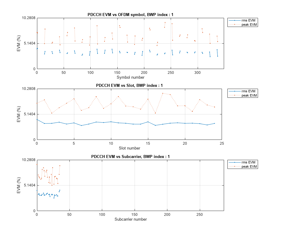


Averaged overall PDSCH RMS EVM: 2.675%
Overall PDSCH Peak EVM = 11.2764%
Averaged overall PDCCH RMS EVM: 3.363%
Overall PDCCH Peak EVM = 9.3461%
The output of the hNRDownlinkEVM function shows that the demodulation of the received waveform is successful.