Active Noise Control Using a Filtered-X LMS FIR Adaptive Filter
This example shows how to apply adaptive filters to the attenuation of acoustic noise via active noise control.
Active Noise Control
In active noise control, one attempts to reduce the volume of an unwanted noise propagating through the air using an electro-acoustic system using measurement sensors such as microphones and output actuators such as loudspeakers. The noise signal usually comes from some device, such as a rotating machine, so that it is possible to measure the noise near its source. The goal of the active noise control system is to produce an "anti-noise" that attenuates the unwanted noise in a desired quiet region using an adaptive filter. This problem differs from traditional adaptive noise cancellation in that: - The desired response signal cannot be directly measured; only the attenuated signal is available. - The active noise control system must take into account the secondary loudspeaker-to-microphone error path in its adaptation.
For more implementation details on active noise control tasks, see S.M. Kuo and D.R. Morgan, "Active Noise Control Systems: Algorithms and DSP Implementations", Wiley-Interscience, New York, 1996.
The Secondary Propagation Path
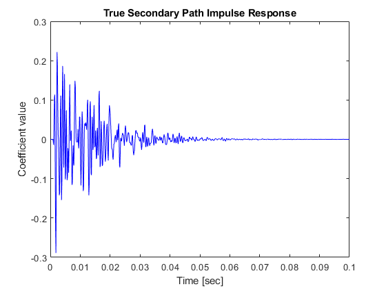
The secondary propagation path is the path the anti-noise takes from the output loudspeaker to the error microphone within the quiet zone. The following commands generate a loudspeaker-to-error microphone impulse response that is bandlimited to the range 160 - 2000 Hz and with a filter length of 0.1 seconds. For this active noise control task, we shall use a sampling frequency of 8000 Hz.
Fs     = 8e3;  % 8 kHz
N      = 800;  % 800 samples@8 kHz = 0.1 seconds
Flow   = 160;  % Lower band-edge: 160 Hz
Fhigh  = 2000; % Upper band-edge: 2000 Hz
delayS = 7;
Ast    = 20;   % 20 dB stopband attenuation
Nfilt  = 8;    % Filter order

% Design bandpass filter to generate bandlimited impulse response
filtSpecs = fdesign.bandpass('N,Fst1,Fst2,Ast',Nfilt,Flow,Fhigh,Ast,Fs);
bandpass = design(filtSpecs,'cheby2','FilterStructure','df2tsos', ...
    'SystemObject',true);

% Filter noise to generate impulse response
secondaryPathCoeffsActual = bandpass([zeros(delayS,1); ...
                       log(0.99*rand(N-delayS,1)+0.01).* ...
                       sign(randn(N-delayS,1)).*exp(-0.01*(1:N-delayS)')]);
secondaryPathCoeffsActual = ...
    secondaryPathCoeffsActual/norm(secondaryPathCoeffsActual);

t = (1:N)/Fs;
plot(t,secondaryPathCoeffsActual,'b');
xlabel('Time [sec]');
ylabel('Coefficient value');
title('True Secondary Path Impulse Response');

Estimating the Secondary Propagation Path
The first task in active noise control is to estimate the impulse response of the secondary propagation path. This step is usually performed prior to noise control using a synthetic random signal played through the output loudspeaker while the unwanted noise is not present. The following commands generate 3.75 seconds of this random noise as well as the measured signal at the error microphone.
ntrS = 30000;
randomSignal = randn(ntrS,1); % Synthetic random signal to be played
secondaryPathGenerator = dsp.FIRFilter('Numerator',secondaryPathCoeffsActual.');
secondaryPathMeasured = secondaryPathGenerator(randomSignal) + ... % random signal propagated through secondary path
    0.01*randn(ntrS,1); % measurement noise at the microphone
Designing the Secondary Propagation Path Estimate
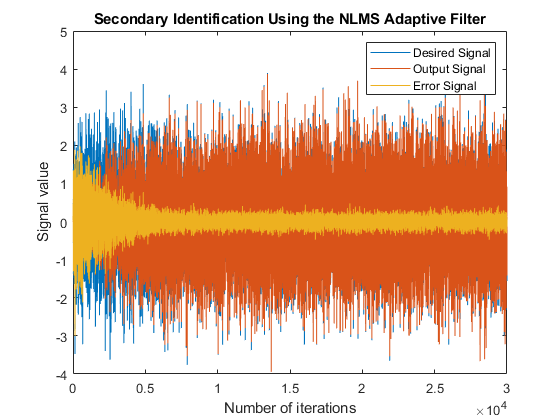
Typically, the length of the secondary path filter estimate is not as long as the actual secondary path and need not be for adequate control in most cases. We shall use a secondary path filter length of 250 taps, corresponding to an impulse response length of 31 ms. While any adaptive FIR filtering algorithm could be used for this purpose, the normalized LMS algorithm is often used due to its simplicity and robustness. Plots of the output and error signals show that the algorithm converges after about 10000 iterations.
M = 250;
muS = 0.1;
secondaryPathEstimator = dsp.LMSFilter('Method','Normalized LMS','StepSize', muS, ...
    'Length', M);
[yS,eS,SecondaryPathCoeffsEst] = secondaryPathEstimator(randomSignal,secondaryPathMeasured);

n = 1:ntrS;
figure, plot(n,secondaryPathMeasured,n,yS,n,eS);
xlabel('Number of iterations');
ylabel('Signal value');
title('Secondary Identification Using the NLMS Adaptive Filter');
legend('Desired Signal','Output Signal','Error Signal');

Accuracy of the Secondary Path Estimate
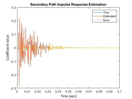
How accurate is the secondary path impulse response estimate? This plot shows the coefficients of both the true and estimated path. Only the tail of the true impulse response is not estimated accurately. This residual error does not significantly harm the performance of the active noise control system during its operation in the chosen task.
figure, plot(t,secondaryPathCoeffsActual, ...
    t(1:M),SecondaryPathCoeffsEst, ...
    t,[secondaryPathCoeffsActual(1:M)-SecondaryPathCoeffsEst(1:M); secondaryPathCoeffsActual(M+1:N)]);
xlabel('Time [sec]');
ylabel('Coefficient value');
title('Secondary Path Impulse Response Estimation');
legend('True','Estimated','Error');

The Primary Propagation Path
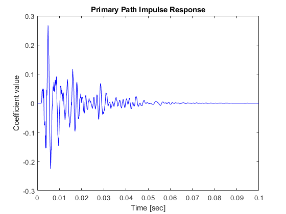
The propagation path of the noise to be canceled can also be characterized by a linear filter. The following commands generate an input-to-error microphone impulse response that is bandlimited to the range 200 - 800 Hz and has a filter length of 0.1 seconds.
delayW = 15;
Flow   = 200; % Lower band-edge: 200 Hz
Fhigh  = 800; % Upper band-edge: 800 Hz
Ast    = 20;  % 20 dB stopband attenuation
Nfilt  = 10;  % Filter order

% Design bandpass filter to generate bandlimited impulse response
filtSpecs2 = fdesign.bandpass('N,Fst1,Fst2,Ast',Nfilt,Flow,Fhigh,Ast,Fs);
bandpass2 = design(filtSpecs2,'cheby2','FilterStructure','df2tsos', ...
    'SystemObject',true);

% Filter noise to generate impulse response
primaryPathCoeffs = bandpass2([zeros(delayW,1); log(0.99*rand(N-delayW,1)+0.01).* ...
    sign(randn(N-delayW,1)).*exp(-0.01*(1:N-delayW)')]);
primaryPathCoeffs = primaryPathCoeffs/norm(primaryPathCoeffs);

figure, plot(t,primaryPathCoeffs,'b');
xlabel('Time [sec]');
ylabel('Coefficient value');
title('Primary Path Impulse Response');

The Noise to Be Canceled
Typical active noise control applications involve the sounds of rotating machinery due to their annoying characteristics. Here, we synthetically generate noise that might come from a typical electric motor.
Initialization of Active Noise Control
The most popular adaptive algorithm for active noise control is the filtered-X LMS algorithm. This algorithm uses the secondary path estimate to calculate an output signal whose contribution at the error sensor destructively interferes with the undesired noise. The reference signal is a noisy version of the undesired sound measured near its source. We shall use a controller filter length of about 44 ms and a step size of 0.0001 for these signal statistics.
% FIR Filter to be used to model primary propagation path
primaryPathGenerator = dsp.FIRFilter('Numerator',primaryPathCoeffs.');

% Filtered-X LMS adaptive filter to control the noise
L = 350;
muW = 0.0001;
noiseController = dsp.FilteredXLMSFilter('Length',L,'StepSize',muW, ...
    'SecondaryPathCoefficients',SecondaryPathCoeffsEst);

% Sine wave generator to synthetically create the noise
A = [.01 .01 .02 .2 .3 .4 .3 .2 .1 .07 .02 .01];
La = length(A);
F0 = 60;
k = 1:La;
F = F0*k;
phase = rand(1,La); % Random initial phase
sine = audioOscillator('NumTones', La, 'Amplitude',A,'Frequency',F, ...
    'PhaseOffset',phase,'SamplesPerFrame',512,'SampleRate',Fs);

% Audio player to play noise before and after cancellation
player = audioDeviceWriter('SampleRate',Fs);

% Spectrum analyzer to show original and attenuated noise
scope = spectrumAnalyzer('SampleRate',Fs, ...
    'PlotAsTwoSidedSpectrum',false, ...
    'ShowLegend',true, ...
    'ChannelNames', {'Original noisy signal', 'Attenuated noise'});
Simulation of Active Noise Control Using the Filtered-X LMS Algorithm
Here we simulate the active noise control system. To emphasize the difference we run the system with no active noise control for the first 200 iterations. Listening to its sound at the error microphone before cancellation, it has the characteristic industrial "whine" of such motors.
Once the adaptive filter is enabled, the resulting algorithm converges after about 5 (simulated) seconds of adaptation. Comparing the spectrum of the residual error signal with that of the original noise signal, we see that most of the periodic components have been attenuated considerably. The steady-state cancellation performance may not be uniform across all frequencies, however. Such is often the case for real-world systems applied to active noise control tasks. Listening to the error signal, the annoying "whine" is reduced considerably.
for m = 1:400
    % Generate synthetic noise by adding sine waves with random phase
    x = sine();
    d = primaryPathGenerator(x) + ...  % Propagate noise through primary path
        0.1*randn(size(x)); % Add measurement noise
    if m <= 200
        % No noise control for first 200 iterations
        e = d;
    else
        % Enable active noise control after 200 iterations
        xhat = x + 0.1*randn(size(x));
        [y,e] = noiseController(xhat,d);
    end
    player(e);     % Play noise signal
    scope([d,e]); % Show spectrum of original (Channel 1)
                     % and attenuated noise (Channel 2)
end
release(player); % Release audio device
release(scope); % Release spectrum analyzer
