Control of a Linear Electric Actuator

This example shows how to use slTuner and systune to tune the current and velocity loops in a linear electric actuator with saturation limits.

Linear Electric Actuator Model

Open the Simulink® model of the linear electric actuator:

open_system('rct_linact')

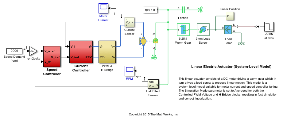
The electrical and mechanical components are modeled using Simscape™ Electrical™. The control system consists of two cascaded feedback loops controlling the driving current and angular speed of the DC motor.

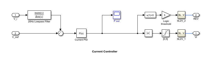
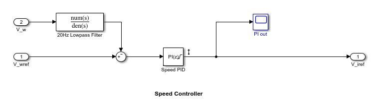
Figure 1: Current and Speed Controllers.

Note that the inner-loop (current) controller is a proportional gain while the outer-loop (speed) controller has proportional and integral actions. The output of both controllers is limited to plus/minus 5.

Design Specifications

We need to tune the proportional and integral gains to respond to a 2000 rpm speed demand in about 0.1 seconds with minimum overshoot. The initial gain settings in the model are P=50 and PI(s)=0.2+0.1/s and the corresponding response is shown in Figure 2. This response is too slow and too sensitive to load disturbances.

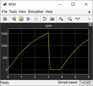
Figure 2: Untuned Response.

Control System Tuning

You can use systune to jointly tune both feedback loops. To set up the design, create an instance of the slTuner interface with the list of tuned blocks. All blocks and signals are specified by their names in the model. The model is linearized at t=0.5 to avoid discontinuities in some derivatives at t=0.

TunedBlocks = {'Current PID','Speed PID'};
tLinearize = 0.5;  % linearize at t=0.5

% Create tuning interface
ST0 = slTuner('rct_linact',TunedBlocks,tLinearize);
addPoint(ST0,{'Current PID','Speed PID'})

The data structure ST0 contains a description of the control system and its tunable elements. Next specify that the DC motor should follow a 2000 rpm speed demand in 0.1 seconds:

TR = TuningGoal.Tracking('Speed Demand (rpm)','rpm',0.1);

You can now tune the proportional and integral gains with systune:

ST1 = systune(ST0,TR);

Final: Soft = 1.04, Hard = -Inf, Iterations = 40

This returns an updated description ST1 containing the tuned gain values. To validate this design, plot the closed-loop response from speed demand to speed:

T1 = getIOTransfer(ST1,'Speed Demand (rpm)',{'rpm','i'});
figure
step(T1,0.5)

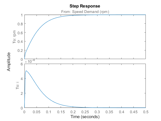
The response looks good in the linear domain so push the tuned gain values to Simulink and further validate the design in the nonlinear model.

writeBlockValue(ST1)

The nonlinear simulation results appear in Figure 3. The nonlinear behavior is far worse than the linear approximation. Figure 4 shows saturation and oscillations in the inner (current) loop.

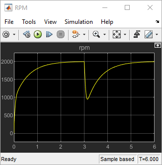
Figure 3: Nonlinear Simulation of Tuned Controller.

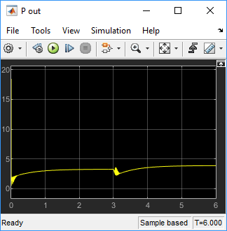
Figure 4: Current Controller Output.

Preventing Saturations

So far we have only specified a desired response time for the outer (speed) loop. This leaves systune free to allocate the control effort between the inner and outer loops. Saturation in the inner loop suggests that the proportional gain is too high and that some rebalancing is needed. One possible remedy is to explicitly limit the gain from the speed command to the "Current PID" output. For a speed reference of 2000 rpm and saturation limits of plus/minus 5, the average gain should not exceed 5/2000 = 0.0025. To be conservative, try keeping the gain from speed reference to "Current PID" below 0.001. To do this, add a gain constraint and retune the controller gains with both requirements in place.

% Mark the "Current PID" output as a point of interest
addPoint(ST0,'Current PID')

% Limit gain from speed demand to "Current PID" output to avoid saturation
MG = TuningGoal.Gain('Speed Demand (rpm)','Current PID',0.001);

% Retune with this additional goal
ST2 = systune(ST0,[TR,MG]);

Final: Soft = 1.39, Hard = -Inf, Iterations = 52

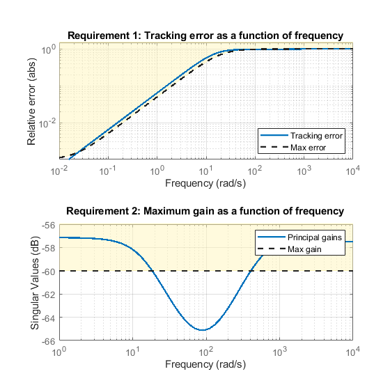
The final gain 1.39 indicates that the requirements are nearly but not exactly met (all requirements are met when the final gain is less than 1). Use viewGoal to inspect how the tuned controllers fare against each goal.

figure('Position',[100,100,560,550])
viewGoal([TR,MG],ST2)

Next compare the two designs in the linear domain.

T2 = getIOTransfer(ST2,'Speed Demand (rpm)',{'rpm','i'});
figure
step(T1,'b',T2,'g--',0.4)
legend('Initial tuning','Tuning with Gain Constraint')

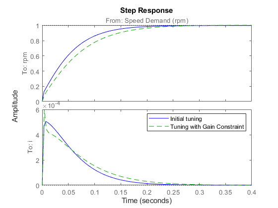
The second design is less aggressive but still meets the response time requirement. A comparison of the tuned PID gains shows that the proportional gain in the current loop was reduced from 18 to about 2.

showTunable(ST1)  % initial tuning

Block 1: rct_linact/Current Controller/Current PID =
 
  Kp = 30
 
Name: Current_PID
P-only controller.

-----------------------------------

Block 2: rct_linact/Speed Controller/Speed PID =
 
             1 
  Kp + Ki * ---
             s 

  with Kp = 0.391, Ki = 0.411
 
Name: Speed_PID
Continuous-time PI controller in parallel form.

showTunable(ST2)  % retuning

Block 1: rct_linact/Current Controller/Current PID =
 
  Kp = 2.19
 
Name: Current_PID
P-only controller.

-----------------------------------

Block 2: rct_linact/Speed Controller/Speed PID =
 
             1 
  Kp + Ki * ---
             s 

  with Kp = 0.482, Ki = 4.96
 
Name: Speed_PID
Continuous-time PI controller in parallel form.

To validate this new design, push the new tuned gain values to the Simulink model and simulate the response to a 2000 rpm speed demand and 500 N load disturbance. The simulation results appear in Figure 5 and the current controller output is shown in Figure 6.

writeBlockValue(ST2)

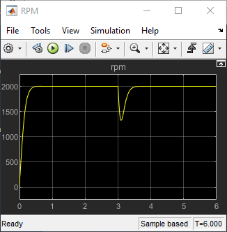
Figure 5: Nonlinear Response of Tuning with Gain Constraint.

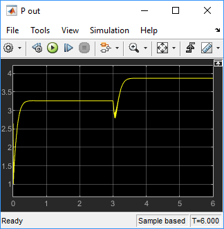
Figure 6: Current Controller Output.

The nonlinear responses are now satisfactory and the current loop is no longer saturating. The additional gain constraint has successfully rebalanced the control effort between the inner and outer loops.