smooth

R2026b

Backward recursion of Bayesian linear state-space model

Since R2026b

Syntax

[X,logL] = smooth(PriorMdl,Y,params)

[X,logL] = smooth(PriorMdl,Y,params,Name=Value)

[X,logL,Output] = smooth(___)

Description

[X,logL] = smooth(PriorMdl,Y,params) returns the means X of the posterior state smoothing distribution for all sampling times in the input response data Y, and the corresponding loglikelihood logL. To return the results, the function performs backward recursion, or smoothing, of the prior Bayesian linear state-space model PriorMdl. smooth computes the posterior distribution of the states conditioned on the state-space model parameters params. This computation does not incorporate parameter uncertainty.

smooth obtains smoothing distribution estimates of a model with Gaussian state disturbances and observation innovations, regardless of the values of the StateDistribution and ObservationDistribution properties of PriorMdl. To sample from the posterior state smoothing distribution of models with non-Gaussian error distributions, see simsmooth.

[X,logL] = smooth(PriorMdl,Y,params,Name=Value) specifies additional options using one or more name-value arguments. For example, smooth(PriorMdl,Y,params,Univariate=true,SquareRoot=true) specifies the univariate treatment of a multivariate state series, and use of the square root filter algorithm of the Kalman filter.

[X,logL,Output] = smooth(___) additionally returns the output structure array Output using any of the input argument combinations in the previous syntaxes. Output contains the following information associated with each observation in the input data:

• Loglikelihood value associated with the input data and parameters

• Smoothed state estimates with uncertainty

• Smoothed estimates of the state disturbances and observation innovations with uncertainty

• Kalman gain matrix

• Flags indicating the data used by the software for smoothing

Examples

Compute Smooth State Estimates and Loglikelihood

Simulate observed responses from a known state-space model, estimate the posterior distribution of the parameters, and then obtain state estimates from the posterior smoothing distribution.

Suppose the following state-space model is a data generating process (DGP).

$$\left[\begin{array}{c}{x}_{t,1}\\ x_{t,2}\end{array}\right]=\left[\begin{array}{cc}0.5& 0\\ 0& -0.75\end{array}\right]\left[\begin{array}{c}{x}_{t-1,1}\\ x_{t-1,2}\end{array}\right]+\left[\begin{array}{cc}1& 0\\ 0& 0.5\end{array}\right]\left[\begin{array}{c}{u}_{t,1}\\ u_{t,2}\end{array}\right]$$

$$y_t=\left[\begin{array}{cc}1& 1\end{array}\right]\left[\begin{array}{c}{x}_{t,1}\\ x_{t,2}\end{array}\right].$$

Create a standard state-space model object ssm that represents the DGP.

trueTheta = [0.5; -0.75; 1; 0.5];
A = [trueTheta(1) 0; 0 trueTheta(2)];
B = [trueTheta(3) 0; 0 trueTheta(4)];
C = [1 1];
DGP = ssm(A,B,C);

Simulate a response path from the DGP, and obtain smoothed state estimates.

rng(1); % For reproducibility
y = simulate(DGP,200);
XSmooth = smooth(DGP,y);

Suppose the structure of the DGP is known, but the state parameters trueTheta are unknown, explicitly

$$\left[\begin{array}{c}{x}_{t,1}\\ x_{t,2}\end{array}\right]=\left[\begin{array}{cc}{\varphi }_1& 0\\ 0& {\varphi }_2\end{array}\right]\left[\begin{array}{c}{x}_{t-1,1}\\ x_{t-1,2}\end{array}\right]+\left[\begin{array}{cc}{\sigma }_1& 0\\ 0& {\sigma }_2\end{array}\right]\left[\begin{array}{c}{u}_{t,1}\\ u_{t,2}\end{array}\right]$$

$$y_t=\left[\begin{array}{cc}1& 1\end{array}\right]\left[\begin{array}{c}{x}_{t,1}\\ x_{t,2}\end{array}\right].$$

Consider a Bayesian state-space model that represents the model with unknown parameters. Assume that the prior distributions of ${\varphi }_1$, ${\varphi }_2$, ${\sigma }_1^2$, and ${\sigma }_2^2$ are independent Gaussian with mean 0.5 and variance 1.

The Local Functions section contains two functions required to specify the Bayesian state-space model. You can use the functions only within this script.

The paramMap function accepts a vector of the unknown state-space model parameters and returns all the following quantities:

• A = $\left[\begin{array}{cc}{\varphi }_1& 0\\ 0& {\varphi }_2\end{array}\right]$.

• B = $\left[\begin{array}{cc}{\sigma }_1& 0\\ 0& {\sigma }_2\end{array}\right]$.

• C = $\left[\begin{array}{cc}1& 1\end{array}\right]$.

• D = 0.

• Mean0 and Cov0 are empty arrays [], which specify the defaults.

• StateType = $\left[\begin{array}{cc}0& 0\end{array}\right]$, indicating that each state is stationary.

The priorDistribution function accepts the same vector of unknown parameters, but returns the log prior density of the parameters at their current values. The function specifies that parameter values outside the parameter space have a log prior density of -Inf.

Create the Bayesian state-space model by passing function handles for paramMap and priorDistribution directly to bssm.

PriorMdl = bssm(@paramMap,@priorDistribution)

PriorMdl = 
Mapping that defines a state-space model:
    @paramMap

Log density of parameter prior distribution:
    @priorDistribution

PriorMdl is a bssm object representing the Bayesian state-space model with unknown parameters.

Estimate the posterior distribution using estimate. Specify a random set of positive values in [0,1] to initialize the Markov chain Monte Carlo (MCMC) algorithm. Tune the sampler by applying a 500 burn-in period, thinning the sample by a factor of 30, and obtaining 2000 draws (after processing). Return parameter estimates from the posterior distribution.

numParams = 4;
theta0 = rand(numParams,1);
[PosteriorMdl,estParams] = estimate(PriorMdl,y,theta0,Univariate=true, ...
    BurnIn=500,NumDraws=2000,Thin=30);

Local minimum found.

Optimization completed because the size of the gradient is less than
the value of the optimality tolerance.

<stopping criteria details>
         Optimization and Tuning        
      | Params0  Optimized  ProposalStd 
----------------------------------------
 c(1) |  0.6968    0.4459      0.0798   
 c(2) |  0.7662   -0.8781      0.0483   
 c(3) |  0.3425    0.9633      0.0694   
 c(4) |  0.8459    0.3978      0.0726   
 
             Posterior Distributions            
      |   Mean     Std   Quantile05  Quantile95 
------------------------------------------------
 c(1) |  0.4495  0.0822     0.3135      0.5858  
 c(2) | -0.8561  0.0587    -0.9363     -0.7468  
 c(3) |  0.9645  0.0744     0.8448      1.0863  
 c(4) |  0.4333  0.0860     0.3086      0.5889  
Proposal acceptance rate = 38.85%

PosteriorMdl is a bssm object representing the posterior distribution.

Obtain state estimates from the posterior smoothing distribution and return the data loglikelihood.

[XSmoothHat,logL] = smooth(PosteriorMdl,y,estParams);

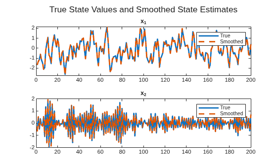
Plot the state estimates with the true values.

figure
tiledlayout(2,1)
nexttile
plot(XSmooth(:,1),"-",LineWidth=2)
hold on
plot(XSmoothHat(:,1),"--",LineWidth=2)
hold off
title("x_1")
legend("True","Smoothed")
nexttile
plot(XSmooth(:,2),"-",LineWidth=2)
hold on
plot(XSmoothHat(:,2),"--",LineWidth=2)
hold off
title("x_2")
legend("True","Smoothed")
sgtitle("True State Values and Smoothed State Estimates")

Local Functions

This example uses the following functions. paramMap is the parameter-to-matrix mapping function, and priorDistribution is the log prior distribution of the parameters.

function [A,B,C,D,Mean0,Cov0,StateType] = paramMap(theta)
    A = [theta(1) 0; 0 theta(2)];
    B = [theta(3) 0; 0 theta(4)];
    C = [1 1];
    D = 0;              % No observation noise
    Mean0 = [];         % MATLAB uses default initial state mean
    Cov0 = [];          % MATLAB uses default initial state covariances
    StateType = [0; 0]; % Two stationary states
end

function logprior = priorDistribution(theta)
    paramconstraints = [(abs(theta(1)) >= 1) (abs(theta(2)) >= 1) ...
        (theta(3) < 0) (theta(4) < 0)];
    if(sum(paramconstraints))
        logprior = -Inf;
    else 
        mu0 = 0.5*ones(numel(theta),1); 
        sigma0 = 1;
        p = normpdf(theta,mu0,sigma0);
        logprior = sum(log(p));
    end
end

Obtain Smoothed Coefficient Estimates of Regression Equation

Model the coefficients of a linear regression as a random walk within a Bayesian state-space model. Track the evolution of the coefficients as the system processes observations.

The Bayesian state-space model is

$$\begin{array}{l}{y}_t={\beta }_{0,t}+{\beta }_{1,t}{x}_{1,t}+{\beta }_{2,t}{x}_{2,t}+u_t\\ {\beta }_t={\beta }_{t-1}+{\epsilon }_t,\end{array}$$

where:

• $y_t$ is the US three-month T-bill rate.

• $x_{1,t}$ is the US CPI-based inflation rate.

• $x_{2,t}$ is the US M2 money supply growth rate.

• ${\beta }_t=\left[\begin{array}{ccc}{\beta }_{0,t}& {\beta }_{1,t}& {\beta }_{2t}\end{array}\right]\prime$ is the vector of coefficients.

• ${\epsilon }_t$ is a series of 3-D iid Gaussian disturbances. The variance of dimension $j$ is ${\sigma }_j^2$ and the prior distribution of ${\sigma }_j^2$ is $IG\left(2,0.5\right)$.

• $u_t$ is an iid Gaussian innovation series. The variance is ${\sigma }_4^2$ and the prior distribution of ${\sigma }_4^2$ is $IG\left(2,0.5\right)$.

Load the US macroeconomic data Data_USEconModel.mat. The variable DataTimeTable is a timetable that contains the series in the regression model, among other series. Extract the response and predictor variables CPIAUCSL, M2SL, and TB3MS, and remove all observations that contain at least one missing value.

load Data_USEconModel
DTT = rmmissing(DataTimeTable(:,["CPIAUCSL" "M2SL" "TB3MS"]));

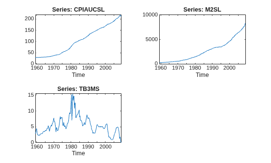
Plot the series separately.

figure
tiledlayout(2,2)
for j = 1:3
    nexttile
    plot(DTT.Time,DTT{:,j})
    title("Series: " + DTT.Properties.VariableNames{j})
    xlabel("Time")
end

Stabilize the series by applying the first difference to the three-month T-bill series, and by converting the predictor series to rates.

y = diff(DTT.TB3MS);
X = DTT{:,["CPIAUCSL" "M2SL"]};
X = price2ret(X);

The Local Functions section contains two functions required to specify the Bayesian state-space model. You can use the functions only within this script.

The paramMap function accepts a vector of the four variances in the state-space model, the predictor data X, and the sample size $T$, and returns the following quantities:

• $A=\left[\begin{array}{ccc}1& 0& 0\\ 0& 1& 0\\ 0& 0& 1\end{array}\right]$.

• $B=\left[\begin{array}{ccc}{\sigma }_1& 0& 0\\ 0& {\sigma }_2& 0\\ 0& 0& {\sigma }_3\end{array}\right]$.

• $C$ is a $T$-by-1 cell vector, where cell $t$ is $x_t\prime {\beta }_t$.

• $D={\sigma }_4$.

• Mean0 and Cov0 are empty arrays [], which specify the defaults.

• StateType = $\left[\begin{array}{ccc}2& 2& 2\end{array}\right]\prime$, indicating that each state is nonstationary.

The priorDistribution function accepts the same vector of unknown parameters, but returns the log prior density of the parameters at their current values. The function specifies that parameter values outside the parameter space have a log prior density of -Inf.

Create the Bayesian state-space model by passing function handles for paramMap and priorDistribution directly to bssm. Determine the sample size $T$, and set the shape and scale of the inverse gamma distribution to variables.

T = numel(y);
a = 2.0; 
b = 0.5; 
PriorMdl = bssm(@(theta)paramMap(theta,X,T),@(theta)priorDistribution(theta,a,b));

PriorMdl is a bssm object representing the Bayesian state-space model.

Fit the model to the data. Choose the initial state of the parameters randomly from $IG\left(2,0.5\right)$. Because the observation innovations are uncorrelated, set the univariate treatment of the multivariate model for computational efficiency. For numerical stability, apply the square root filter.

rng(1,"twister")
params0 = 1./gamrnd(a,b,4,1);
[PosteriorMdl,estParams] = estimate(PriorMdl,y,params0, ...
    Univariate=true,Squareroot=true)

Local minimum found.

Optimization completed because the size of the gradient is less than
the value of the optimality tolerance.

<stopping criteria details>
         Optimization and Tuning        
      | Params0  Optimized  ProposalStd 
----------------------------------------
 c(1) |  0.5400    0.0705      0.0209   
 c(2) |  5.5331    0.1663      0.0957   
 c(3) |  3.3037    0.1663      0.0957   
 c(4) |  1.9393    1.0591      0.0537   
 
            Posterior Distributions            
      |  Mean     Std   Quantile05  Quantile95 
-----------------------------------------------
 c(1) | 0.0771  0.0198    0.0488      0.1114   
 c(2) | 0.2858  0.1441    0.1046      0.5602   
 c(3) | 0.3139  0.1816    0.1033      0.6640   
 c(4) | 1.0640  0.0577    0.9741      1.1538   
Proposal acceptance rate = 42.10%

PosteriorMdl = 
  bssm with properties:

                   ParamMap: @(theta)paramMap(theta,X,T)
          ParamDistribution: [4×1000 double]
          StateDistribution: [1×1 struct]
    ObservationDistribution: [1×1 struct]

            Posterior Distributions            
      |  Mean     Std   Quantile05  Quantile95 
-----------------------------------------------
 c(1) | 0.0771  0.0198    0.0488      0.1114   
 c(2) | 0.2858  0.1441    0.1046      0.5602   
 c(3) | 0.3139  0.1816    0.1033      0.6640   
 c(4) | 1.0640  0.0577    0.9741      1.1538   

State-space model type: ssm

State vector length: 3
Observation vector length: 1
State disturbance vector length: 3
Observation innovation vector length: 1
Sample size supported by model: 200

State variables: x1, x2,...
State disturbances: u1, u2,...
Observation series: y1, y2,...
Observation innovations: e1, e2,...

State equations:
x1(t) = x1(t-1) + (0.08)u1(t)
x2(t) = x2(t-1) + (0.29)u2(t)
x3(t) = x3(t-1) + (0.31)u3(t)

Observation equation of period 1:
y1(t) = x1(t) + (4.82e-03)x2(t) + (0.02)x3(t) + (1.06)e1(t)

Observation equation of period 2:
y1(t) = x1(t) + (4.80e-03)x2(t) + (8.80e-03)x3(t) + (1.06)e1(t)

Observation equation of period 3:
y1(t) = x1(t) + (5.46e-03)x2(t) + (3.70e-03)x3(t) + (1.06)e1(t)

Observation equation of period 4:
y1(t) = x1(t) + (5.36e-03)x3(t) + (1.06)e1(t)

Observation equation of period 5:
y1(t) = x1(t) + (6.78e-03)x2(t) + (9.64e-03)x3(t) + (1.06)e1(t)

Observation equation of period 6:
y1(t) = x1(t) + (0.02)x3(t) + (1.06)e1(t)

Observation equation of period 7:
y1(t) = x1(t) + (6.73e-03)x2(t) + (0.01)x3(t) + (1.06)e1(t)

Observation equation of period 8:
y1(t) = x1(t) + (1.01e-03)x2(t) + (0.02)x3(t) + (1.06)e1(t)

Observation equation of period 9:
y1(t) = x1(t) + (0.02)x3(t) + (1.06)e1(t)

Observation equation of period 10:
y1(t) = x1(t) + (4.68e-03)x2(t) + (0.02)x3(t) + (1.06)e1(t)

... (Set 'Period' parameter to see intermediate equations)

Observation equation of period 191:
y1(t) = x1(t) + (2.46e-03)x2(t) + (0.02)x3(t) + (1.06)e1(t)

Observation equation of period 192:
y1(t) = x1(t) + (0.01)x2(t) + (0.01)x3(t) + (1.06)e1(t)

Observation equation of period 193:
y1(t) = x1(t) + (8.12e-03)x2(t) + (0.01)x3(t) + (1.06)e1(t)

Observation equation of period 194:
y1(t) = x1(t) + (6.54e-03)x2(t) + (0.02)x3(t) + (1.06)e1(t)

Observation equation of period 195:
y1(t) = x1(t) + (0.02)x2(t) + (0.01)x3(t) + (1.06)e1(t)

Observation equation of period 196:
y1(t) = x1(t) + (9.07e-03)x2(t) + (0.02)x3(t) + (1.06)e1(t)

Observation equation of period 197:
y1(t) = x1(t) + (0.02)x2(t) + (6.44e-03)x3(t) + (1.06)e1(t)

Observation equation of period 198:
y1(t) = x1(t) + (7.53e-03)x2(t) + (0.02)x3(t) + (1.06)e1(t)

Observation equation of period 199:
y1(t) = x1(t) - (0.03)x2(t) + (0.04)x3(t) + (1.06)e1(t)

Observation equation of period 200:
y1(t) = x1(t) + (5.36e-03)x2(t) + (0.02)x3(t) + (1.06)e1(t)


Initial state distribution:

Initial state means
 x1  x2  x3 
  0   0   0 

Initial state covariance matrix
     x1     x2     x3    
 x1  1e+07  0      0     
 x2  0      1e+07  0     
 x3  0      0      1e+07 

State types
    x1       x2       x3   
 Diffuse  Diffuse  Diffuse 

estParams = 4×1

    0.0771
    0.2858
    0.3139
    1.0640

Obtain posterior estimates from the smoothing distribution of the regression coefficients. Apply the univariate treatment and the square root filter.

BetaSmooth = smooth(PosteriorMdl,y,estParams,Univariate=true,SquareRoot=true);

BetaSmooth is a $T$-by-3 matrix containing the posterior estimates of the smoothing distribution of the regression coefficients.

Display the evolution of the coefficient estimates. Plot the estimates separately.

figure
tiledlayout(2,2)
nexttile
plot(BetaSmooth(:,1))
title("\beta_{0,t}")
nexttile
plot(BetaSmooth(:,2))
title("\beta_{1,t}")
nexttile
plot(BetaSmooth(:,3))
title("\beta_{2,t}")

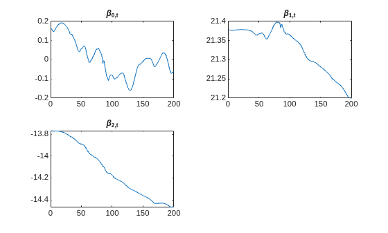
The posterior estimates appear nonstationary, but their values remain within relatively tight intervals.

Compare the final estimates to the estimates from fitting a standard linear model.

Mdl = fitlm(X,y);
[Mdl.Coefficients.Estimate BetaSmooth(end,:)']

ans = 3×2

   -0.0061   -0.0612
   20.2826   21.1997
  -12.4488  -14.4608

The estimates are in fair agreement.

Local Functions

This example uses the following functions. paramMap is the parameter-to-matrix mapping function, and priorDistribution is the log prior distribution of the parameters.

function [A,B,C,D,Mean0,Cov0,StateType] = paramMap(theta,Z,T)
    A = eye(3);
    B = diag(theta(1:3));
    C = cell(T,1);
    for t = 1:T
        C{t} = [1 Z(t,:)];
    end
    D = theta(4);
    Mean0 = [];            % MATLAB uses default initial state mean
    Cov0 = [];             % MATLAB uses default initial state covariances
    StateType = [2; 2; 2]; % Three nonstationary states
end

function logprior = priorDistribution(theta,a,b)
    paramconstraints = theta < 0;
    if(sum(paramconstraints))
        logprior = -Inf;
    else 
        p = zeros(4,1);
        for j = 1:numel(p)
            p(j) = a*log(b) - gammaln(a) - (a+1)*log(theta(j)) - b./theta(j);
        end
        logprior = sum(p);
    end
end

Obtain Smoothed State Estimate Variances

Obtain state smoothing posterior distribution covariances of the regression coefficients in the model from the example Obtain Smoothed Coefficient Estimates of Regression Equation.

Load and preprocess the US macroeconomic data, and then create and estimate the Bayesian state-space model.

load Data_USEconModel
DTT = rmmissing(DataTimeTable(:,["CPIAUCSL" "M2SL" "TB3MS"]));
y = diff(DTT.TB3MS);
X = DTT{:,["CPIAUCSL" "M2SL"]};
X = price2ret(X)*100;
T = numel(y);
a = 2.0; 
b = 0.5; 
PriorMdl = bssm(@(theta)paramMap(theta,X,T),@(theta)priorDistribution(theta,a,b));

rng(100,"twister")
params0 = 1./gamrnd(a,b,4,1);
options = optimoptions("fminunc",Display="off");
[PosteriorMdl,estParams] = estimate(PriorMdl,y,params0, ...
    Univariate=true,SquareRoot=true,Display=false,Options=options);

Obtain posterior estimates from the smoothing distribution of the regression coefficients. Apply the univariate treatment and the square root filter. Return the output structure that contains posterior estimates and variances, and extract the state smoothing posterior distribution covariances into a cell vector.

[BetaSmooth,~,out] = smooth(PosteriorMdl,y,estParams,Univariate=true,SquareRoot=true);
BetaSmoothCov = {out.SmoothedStatesCov};

BetaSmoothCov is a T-by-1 cell vector, where cell $t$ contains the 3-by-3 covariance matrix of the regression coefficients based on the state smoothing posterior distribution.

Plot approximate 95% confidence ellipse projections for the smoothed regression coefficient estimates of the final period in the sample by passing the smooth estimates and t = T (200) to the local function plotConfEllipseProjBeta (see Local Functions). To see confidence ellipses for different values of t, use the control.

t = 200;
plotConfEllipseProjBeta(BetaSmooth,BetaSmoothCov,t)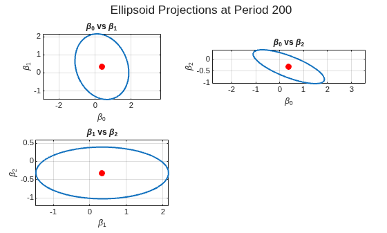

Local Functions

This example uses the following functions. paramMap is the parameter-to-matrix mapping function, priorDistribution is the log prior distribution of the parameters, and plotConfEllipseProjBeta plots confidence ellipses of the coefficients.

function [A,B,C,D,Mean0,Cov0,StateType] = paramMap(theta,Z,T)
    A = eye(3);
    B = diag(theta(1:3));
    C = cell(T,1);
    for t = 1:T
        C{t} = [1 Z(t,:)];
    end
    D = theta(4);
    Mean0 = [];            % MATLAB uses default initial state mean
    Cov0 = [];             % MATLAB uses default initial state covariances
    StateType = [2; 2; 2]; % Three nonstationary states
end

function logprior = priorDistribution(theta,a,b)
    paramconstraints = theta < 0;
    if(sum(paramconstraints))
        logprior = -Inf;
    else 
        p = zeros(4,1);
        for j = 1:numel(p)
            p(j) = a*log(b) - gammaln(a) - (a+1)*log(theta(j)) - b./theta(j);
        end
        logprior = sum(p);
    end
end

function plotConfEllipseProjBeta(est,covar,t)
    p = width(est);
    alpha = 0.05;
    chi2val = chi2inv(1-alpha,p); 
    theta = linspace(0,2*pi,100);
    unitCircle = [cos(theta); sin(theta)];
    mn = est(t,:).';
    Sigma = covar{t}; 
    pairs = nchoosek(1:p,2);
    numpairs = height(pairs);
    projs = cell(numpairs,1);
    for k = 1:numpairs
        idx = pairs(k,:);
        S2 = Sigma(idx,idx);
        S2 = (S2+S2')/2;
        [V,D] = eig(S2);
        D = diag(max(diag(D),0));
        A = V*sqrt(D)*sqrt(chi2val);
        pts = (A*unitCircle) + mn(idx);
        projs{k} = pts.';
    end
    betas = "\beta_" + string(0:(p-1));
    pairNames = betas(pairs);
    titles = join(pairNames, " vs ");
    tiledlayout("flow",Padding="compact",TileSpacing="compact");
    for k = 1:numpairs
        nexttile
        P = projs{k};
        plot(P(:,1),P(:,2),"-",LineWidth=1.5)
        hold on
        plot(mn(pairs(k,1)),mn(pairs(k,2)),"r.",MarkerSize=20)
        xlabel(betas(pairs(k,1)))
        ylabel(betas(pairs(k,2)))
        title(titles(k))
        axis equal
        grid on
        hold off
    end
    sgtitle("Ellipsoid Projections at Period " + t)
end

Input Arguments

PriorMdl — Prior Bayesian linear state-space model

bssm object

Prior Bayesian linear state-space model, specified as a bssm object returned by bssm or ssm2bssm.

The function handles of the properties PriorMdl.ParamDistribution and PriorMdl.ParamMap determine the prior distribution and the data likelihood, respectively. smooth evaluates PriorMdl.ParamMap at params before computing the state posterior distribution.

smooth ignores the values of the properties StateDistribution and ObservationDistribution of PriorMdl, and assumes that the state disturbances and observation innovations are Gaussian.

Y — Observed response data

numeric matrix | cell vector of numeric vectors

Observed response data, from which smooth forms the posterior distribution, specified as a numeric matrix or a cell vector of numeric vectors.

• If PriorMdl is time invariant with respect to the observation equation, Y is a T-by-n matrix. Each row of the matrix corresponds to a period, and each column corresponds to a particular observation in the model. T is the sample size and n is the number of observations per period. The last row of Y contains the latest observations.

• If PriorMdl is time varying with respect to the observation equation, Y is a T-by-1 cell vector. Y{t} contains an n_t-dimensional vector of observations for period t, where t = 1, ..., T. The corresponding dimensions of the coefficient matrices, outputs of PriorMdl.ParamMap, C{t}, and D{t} must be consistent with the matrix in Y{t} for all periods. The last cell of Y contains the latest observations.

NaN elements indicate missing observations. For details on how the Kalman filter accommodates missing observations, see Algorithms.

Data Types: double | cell

params — State-space model parameters Θ

numeric vector

State-space model parameters Θ used to evaluate the parameter mapping Mdl.ParamMap, specified as a numparams-by-1 numeric vector. Elements of params must correspond to the elements of the first input arguments of PriorMdl.ParamMap and PriorMdl.ParamDistribution.

Usually, you pass either the posterior means of the parameters or a draw from their posterior distribution to params. The second output of estimate contains the posterior means of the parameters, and the first output of simulate contains draws from their posterior distribution.

Data Types: double

Name-Value Arguments

Specify optional pairs of arguments as Name1=Value1,...,NameN=ValueN, where Name is the argument name and Value is the corresponding value. Name-value arguments must appear after other arguments, but the order of the pairs does not matter.

Example: smooth(PriorMdl,Y,params,Univariate=true,SquareRoot=true) specifies the univariate treatment of a multivariate state series and use of the square root filter algorithm of the Kalman filter.

Univariate — Flag for univariate treatment of multivariate series

false (default) | true

Flag for the univariate treatment of a multivariate series, specified as false or true.

Value	Description
true	Applies the univariate treatment of a multivariate series, also known as sequential filtering
false	Does not apply sequential filtering

The univariate treatment can accelerate and improve numerical stability of the Kalman filter. However, all observation innovations must be uncorrelated. That is, D_tD_t' must be diagonal, where D_t (t = 1, ..., T) is the output coefficient matrix D of PriorMdl.ParamMap.

Example: Univariate=true

Data Types: logical

SquareRoot — Flag for square root filter method

false (default) | true

Flag for the square root filter method, specified as false or true.

Value	Description
true	Applies the square root filter method for the Kalman filter
false	Does not apply the square root filter method

If you think the eigenvalues of the filtered state or forecasted observation covariance matrices are close to zero, then specify SquareRoot=true. The square root filter is robust to numerical issues arising from the finite precision of calculations, but requires more computational resources.

Example: SquareRoot=true

Data Types: logical

Tolerance — Forecast uncertainty threshold

0 (default) | nonnegative scalar

Forecast uncertainty threshold, specified as a nonnegative scalar.

If the forecast uncertainty for a particular observation is less than Tolerance during numerical estimation, then the software removes the uncertainty corresponding to the observation from the forecast covariance matrix before its inversion.

To overcome numerical obstacles during estimation, It is best practice to set Tolerance to a small number, such as 1e-15.

Example: Tolerance=1e-15

Data Types: double

Output Arguments

X — Means of posterior state smoothing distribution E(x_t|y₁,…,y_T,Θ)

numeric matrix | cell vector of numeric vectors

Means of the posterior state smoothing distribution E(x_t|y₁,…,y_T,Θ), returned as a T-by-m numeric matrix or a T-by-1 cell vector of numeric vectors.

Each row corresponds to a time point in the sample. The last row contains the latest smoothed states.

If PriorMdl is time invariant, smooth returns a matrix. Each column corresponds to a state variable x_t.

If PriorMdl is time varying, X is a cell vector. Cell t contains a column vector of smoothed state estimates with length m_t. Each column corresponds to a state variable.

logL — Loglikelihood function value

scalar

Loglikelihood function value, returned as a scalar.

Missing observations do not contribute to the loglikelihood.

Output — Smoothing results by period

structure array

Smoothing results by period, returned as a structure array.

Output is a T-by-1 structure, where element t corresponds to the smoothing recursion at time t. The following table describes the fields of Output when Univariate is false (the default). When Univariate is true, the fields are the same, but the values in KalmanGain might vary.

Field	Description	Estimate
LogLikelihood	Scalar loglikelihood objective function value	Not applicable
SmoothedStates	mt-by-1 vector of the smoothed states	$$E\left(x_t|y_1,\mathrm{...},y_T,{\Theta }_t\right)$$
SmoothedStatesCov	mt-by-mt variance-covariance matrix of the smoothed states	$$Var\left(x_t|y_1,\mathrm{...},y_T,{\Theta }_t\right)$$
SmoothedStateDisturb	kt-by-1 vector of the smoothed state disturbances	$$E\left(u_t|y_1,\mathrm{...},y_T,{\Theta }_t\right)$$
SmoothedStateDisturbCov	kt-by-kt variance-covariance matrix of the smoothed state disturbances	$$Var\left(u_t|y_1,\mathrm{...},y_T,{\Theta }_t\right)$$
SmoothedObsInnov	ht-by-1 vector of the smoothed observation innovations	$$E\left({\epsilon }_t|y_1,\mathrm{...},y_T,{\Theta }_t\right)$$
SmoothedObsInnovCov	ht-by-ht variance-covariance matrix of the smoothed observation innovations	$$Var\left({\epsilon }_t|y_1,\mathrm{...},y_T,{\Theta }_t\right)$$
KalmanGain	mt-by-nt adjusted Kalman gain matrix	Not applicable
DataUsed	ht-by-1 logical vector indicating whether the software smooths using a particular observation. For example, if observation i at time t is a NaN, then element i in DataUsed at time t is 0.	Not applicable

Algorithms

smooth computes smoothed state estimates under the following conditions:

• smooth evaluates the state-space model parameters at the input values in params, that is, the smoothing state distribution is conditioned on the specified model parameter values.

• The state-disturbance and observation-innovation distributions are Gaussian, despite the values of the properties PriorMdl.StateDistribution and PriorMdl.ObservationDistribution.

As a result, the computation of the means of the posterior state smoothing distribution amounts to a forward Kalman filter recursion, followed by a backward smoothing recursion, of the state-space model by using the standard Kalman filter. Therefore, this smoothing method does not account for model parameter uncertainty (see the smooth function of the ssm object). To work with more flexible models and incorporate model parameter uncertainty, use simsmooth.

smooth accommodates missing data by not updating the smoothed state estimates that correspond to missing observations. In other words, assume a missing observation at period t. The state forecast for period t based on the previous t – 1 observations is equivalent to the smoothed state estimate for period t during backward smoothing.

Version History

Introduced in R2026b