Estimate Regression Model with ARIMA Errors

This example shows how to estimate the sensitivity of the US Gross Domestic Product (GDP) to changes in the Consumer Price Index (CPI) using estimate.

Load the US macroeconomic data set, Data_USEconModel. Plot the GDP and CPI.

load Data_USEconModel
gdp = DataTimeTable.GDP;
cpi = DataTimeTable.CPIAUCSL;

figure
plot(DataTimeTable.Time,gdp)
title("{\bf US Gross Domestic Product, Q1 in 1947 to Q1 in 2009}")
axis tight

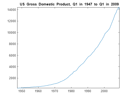
figure
plot(DataTimeTable.Time,cpi)
title("{\bf US Consumer Price Index, Q1 in 1947 to Q1 in 2009}")
axis tight

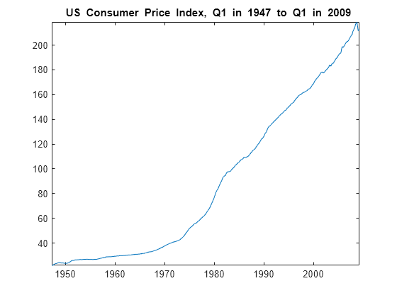
gdp and cpi seem to increase exponentially.

Regress gdp onto cpi. Plot the residuals.

XDes = [ones(length(cpi),1) cpi];   % Design matrix
beta = XDes\gdp;
u = gdp - XDes*beta;                % Residuals

figure
plot(DataTimeTable.Time,u)
h1 = gca;
hold on
plot(h1.XLim,[0 0],"r:")
title("{\bf Residual Plot}")
hold off

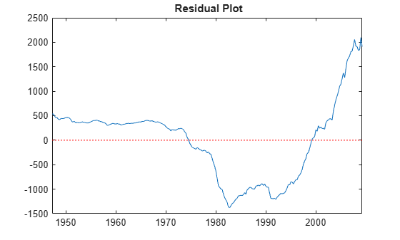
The pattern of the residuals suggests that the standard linear model assumption of uncorrelated errors is violated. The residuals appear autocorrelated.

Plot correlograms for the residuals.

figure
tiledlayout(2,1)
nexttile
autocorr(u)
nexttile
parcorr(u)

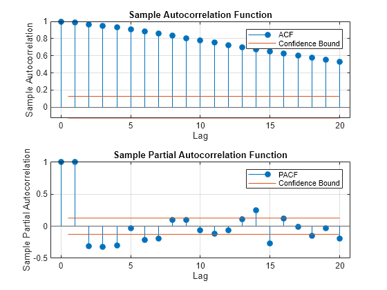
The autocorrelation function suggests that the residuals are a nonstationary process.

Apply the first difference to the logged series to stabilize the residuals.

dlGDP = diff(log(gdp));
dlCPI = diff(log(cpi));
dlXDes = [ones(length(dlCPI),1) dlCPI];
beta = dlXDes\dlGDP;
u = dlGDP - dlXDes*beta;

figure
plot(DataTimeTable.Time(2:end),u);
h2 = gca;
hold on
plot(h2.XLim,[0 0],"r:")
title("{\bf Residual Plot, Transformed Series}")
hold off

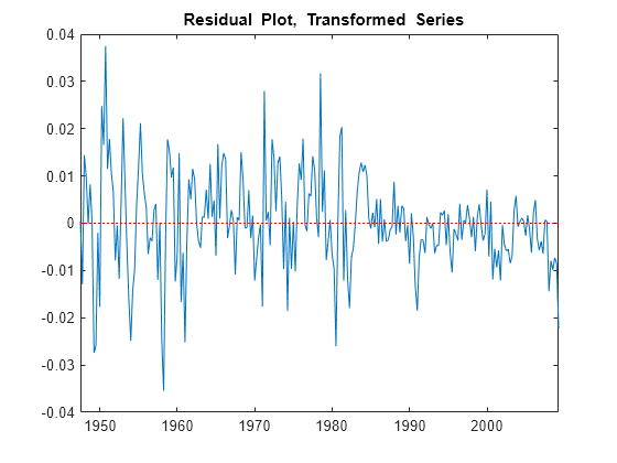
figure
tiledlayout(2,1)
nexttile
autocorr(u)
nexttile
parcorr(u)

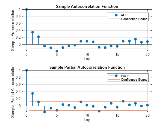
The residual plot from the transformed data suggests stabilized, albeit heteroscedastic, unconditional disturbances. The correlograms suggest that the unconditional disturbances follow an AR(1) process.

Specify the regression model with AR(1) errors:

$$\begin{array}{c}\text{dlGDP}=\text{Intercept}+\text{dlCPI}\beta +u_t\\ u_t=\varphi u_{t-1}+{\epsilon }_t.\end{array}$$

Mdl = regARIMA(ARLags=1);

estimate estimates any parameter having a value of NaN.

Fit Mdl to the data.

EstMdl = estimate(Mdl,dlGDP,X=dlCPI,Display="params");

 
    Regression with ARMA(1,0) Error Model (Gaussian Distribution):
 
                   Value       StandardError    TStatistic      PValue  
                 __________    _____________    __________    __________

    Intercept      0.012762      0.0013472        9.4734      2.7098e-21
    AR{1}           0.38245       0.052494        7.2856      3.2031e-13
    Beta(1)          0.3989       0.077286        5.1614      2.4516e-07
    Variance     9.0101e-05      5.947e-06        15.151      7.5075e-52

Alternatively, estimate the regression coefficients and Newey-West standard errors using hac.

hac(dlCPI,dlGDP,Intercept=true,Display="full");

Estimator type: HAC
Estimation method: BT
Bandwidth: 4.1963
Whitening order: 0
Effective sample size: 248
Small sample correction: on

Coefficient Estimates:

       |  Coeff    SE   
------------------------
 Const | 0.0115  0.0012 
 x1    | 0.5421  0.1005 

Coefficient Covariances:

       |  Const      x1   
--------------------------
 Const |  0.0000  -0.0001 
 x1    | -0.0001   0.0101 

The intercept estimates are close, but the regression coefficient estimates corresponding to dlCPI are not. This is because regARIMA explicitly models for the autocorrelation of the disturbances. hac estimates the coefficients using ordinary least squares, and returns standard errors that are robust to the residual autocorrelation and heteroscedasticity.

Assuming that the model is correct, the results suggest that an increase of one point in the CPI rate increases the GDP growth rate by 0.399 points. This effect is significant according to the t statistic.

From here, you can use forecast or simulate to obtain forecasts and forecast intervals for the GDP rate. You can also compare several models by computing their AIC statistics using aicbic.