Forecast Time-Varying Diffuse State-Space Model

This example shows how to generate data from a known model, fit a diffuse state-space model to the data, and then forecast states and observations states from the fitted model.

Suppose that a latent process comprises an AR(2) and an MA(1) model. There are 50 periods, and the MA(1) process drops out of the model for the final 25 periods. Consequently, the state equation for the first 25 periods is

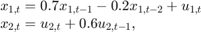
and for the last 25 periods, it is

where and are Gaussian with mean 0 and standard deviation 1.

Assuming that the series starts at 1.5 and 1, respectively, generate a random series of 50 observations from and

T = 50;
ARMdl = arima('AR',{0.7,-0.2},'Constant',0,'Variance',1);
MAMdl = arima('MA',0.6,'Constant',0,'Variance',1);
x0 = [1.5 1; 1.5 1];
rng(1);
x = [simulate(ARMdl,T,'Y0',x0(:,1)),...
    [simulate(MAMdl,T/2,'Y0',x0(:,2));nan(T/2,1)]];

The last 25 values for the simulated MA(1) data are NaN values.

The latent processes are measured using

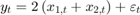
for the first 25 periods, and

for the last 25 periods, where is Gaussian with mean 0 and standard deviation 1.

Use the random latent state process (x) and the observation equation to generate observations.

y = 2*sum(x','omitnan')'+randn(T,1);

Together, the latent process and observation equations make up a state-space model. If the coefficients are unknown parameters, the state-space model is

for the first 25 periods,

for period 26, and

for the last 24 periods.

Write a function that specifies how the parameters in params map to the state-space model matrices, the initial state values, and the type of state.

% Copyright 2015 The MathWorks, Inc.

function [A,B,C,D,Mean0,Cov0,StateType] = diffuseAR2MAParamMap(params,T)
%diffuseAR2MAParamMap Time-variant diffuse state-space model parameter
%mapping function
%
% This function maps the vector params to the state-space matrices (A, B,
% C, and D) and the type of state (StateType). From periods 1 to T/2, the
% state model is an AR(2) and an MA(1) model, and the observation model is
% the sum of the two states. From periods T/2 + 1 to T, the state model is
% just the AR(2) model.  The AR(2) model is diffuse.
    A1 = {[params(1) params(2) 0 0; 1 0 0 0; 0 0 0 params(3); 0 0 0 0]};
    B1 = {[1 0; 0 0; 0 1; 0 1]}; 
    C1 = {params(4)*[1 0 1 0]};
    Mean0 = [];
    Cov0 = [];
    StateType = [2 2 0 0];
    A2 = {[params(1) params(2) 0 0; 1 0 0 0]};
    B2 = {[1; 0]};
    A3 = {[params(1) params(2); 1 0]};
    B3 = {[1; 0]}; 
    C3 = {params(5)*[1 0]};
    A = [repmat(A1,T/2,1);A2;repmat(A3,(T-2)/2,1)];
    B = [repmat(B1,T/2,1);B2;repmat(B3,(T-2)/2,1)];
    C = [repmat(C1,T/2,1);repmat(C3,T/2,1)];
    D = 1;
end

Save this code as a file named diffuseAR2MAParamMap on your MATLAB® path.

Create the diffuse state-space model by passing the function diffuseAR2MAParamMap as a function handle to dssm.

Mdl = dssm(@(params)diffuseAR2MAParamMap(params,T));

dssm implicitly creates the diffuse state-space model. Usually, you cannot verify diffuse state-space models that are implicitly created.

To estimate the parameters, pass the observed responses (y) to estimate. Specify an arbitrary set of positive initial values for the unknown parameters.

params0 = 0.1*ones(5,1);
EstMdl = estimate(Mdl,y,params0);

Method: Maximum likelihood (fminunc)
Effective Sample size:             48
Logarithmic  likelihood:     -110.313
Akaike   info criterion:      230.626
Bayesian info criterion:      240.186
      |     Coeff       Std Err   t Stat     Prob  
---------------------------------------------------
 c(1) |  0.44041       0.27687    1.59069  0.11168 
 c(2) |  0.03949       0.29585    0.13349  0.89380 
 c(3) |  0.78364       1.49222    0.52515  0.59948 
 c(4) |  1.64260       0.66736    2.46134  0.01384 
 c(5) |  1.90409       0.49374    3.85648  0.00012 
      |                                            
      |   Final State   Std Dev    t Stat    Prob  
 x(1) | -0.81932       0.46706   -1.75420  0.07940 
 x(2) | -0.29909       0.45939   -0.65107  0.51500 

EstMdl is a dssm model containing the estimated coefficients. Likelihood surfaces of state-space models might contain local maxima. Therefore, try several initial parameter values, or consider using refine.

Forecast observations and states five periods into the future. Also, obtain measures of variability for the forecasts.

numPeriods = 5;
[fY,yMSE,FX,XMSE] = forecast(EstMdl,numPeriods,y);

forecast uses EstMdl.A{end}, ..., EstMdl.D{end} to forecast the diffuse state-space model. fY and yMSE are numPeriods-by-1 numeric vectors of forecasted observations and variances of the forecasted observations, respectively. FX and XMSE are numPeriods-by-2 matrices of state forecasts and variances of the state forecasts. The columns indicate the state, and the rows indicate the period. For all output arguments, the last row corresponds to the latest forecast.

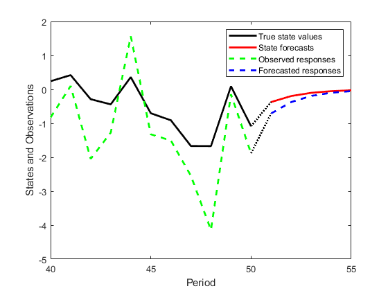
Plot the observations, true states, forecasted observations, and state forecasts.

figure;
plot(T-10:T,x(T-10:T,1),'-k',T+1:T+numPeriods,FX(:,1),'-r',...
    T-10:T,y(T-10:T),'--g',T+1:T+numPeriods,fY,'--b',...
    T:T+1,[y(T),fY(1);x(T,1),FX(1,1)]',':k','LineWidth',2);
xlabel('Period')
ylabel('States and Observations')
legend({'True state values','State forecasts',...
    'Observed responses','Forecasted responses'});