Forecast Univariate Model Responses Using Econometric Modeler App

This example shows how to estimate an ARIMA model and generate forecasts from the model by using the Econometric Modeler app.

Although the example uses an ARIMA model, the workflow is similar for all univariate models available in Econometric Modeler, such as GARCH models. Econometric Modeler cannot forecast models containing exogenous predictor variables, such as ARIMAX models.

The data set, which is stored in Data_JAustralian.mat, contains the log quarterly Australian Consumer Price Index (CPI) measured from 1972 and 1991, among other time series.

Prepare Data for Econometric Modeler

At the command line, load the Data_JAustralian.mat data set.

load Data_JAustralian

Import Data into Econometric Modeler

At the command line, open the Econometric Modeler app.

econometricModeler

Alternatively, open the app from the apps gallery (see Econometric Modeler).

Import DataTimeTable into the app:

1. On the Modeler tab, in the Import section, click the Import button .

2. In the Import Data dialog box, select the check box for the DataTimeTable variable.

3. Click Import.

The variables, including PAU, appear in the Time Series pane, and a time series plot of all the series appears in the Plot(EXCH) figure window.

Create a time series plot of PAU by double-clicking PAU in the Time Series pane.

The series appears nonstationary because it has a clear upward trend.

Specify and Estimate ARIMA Model

Estimate an ARIMA(2,1,0) model containing a constant for the log quarterly Australian CPI. This model has one degree of nonseasonal differencing and two AR lags. For more details, see Implement Box-Jenkins Model Selection and Estimation Using Econometric Modeler App.

1. In the Time Series pane, select the PAU time series.

2. On the Modeler tab, in the Models section, click ARIMA.

3. In the ARIMA Model Parameters dialog box, on the Lag Order tab:

   1. Set Degree of Integration to 1.

   2. Set Autoregressive Order to 2.

   3. Set Moving Average Order to 0.

   

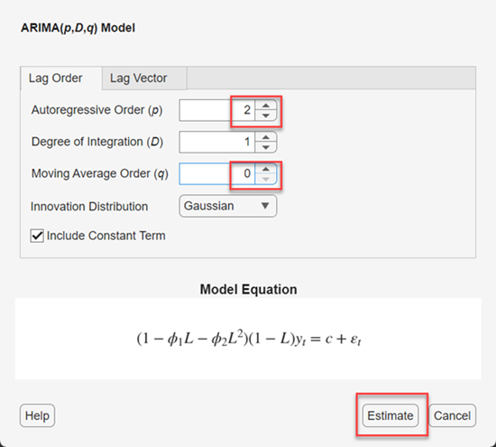
4. Click Estimate.

The model variable ARIMA_PAU appears in the Models pane, its value appears in the Preview pane, and its estimation summary appears in the Fit(ARIMA_PAU) document.

Forecast the Nonstationary Model

Generate MMSE forecasts into a 10-year (40-period) horizon from the nonstationary model.

1. In the Models pane, select the ARIMA_PAU model.

2. On the Modeler tab, in the Forecast section, click Forecast.

3. In the Forecast Model Response dialog box, set Number of periods in forecast horizon to 40. Click Forecast.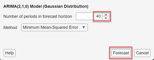

   

In the Forecasts pane, a variable FOR_ARIMA_PAU appears. This variable is a structure array with the following fields:

• Forecast — fh-by-1 vector of forecasted responses, with rows corresponding to the fh specified periods in the forecast horizon

• UpperConfidenceBound — fh-by-1 vector of upper confidence bounds of the pointwise 95% Wald-based forecast intervals

• LowerConfidenceBound — fh-by-1 vector of lower confidence bounds of the pointwise 95% Wald-based forecast intervals

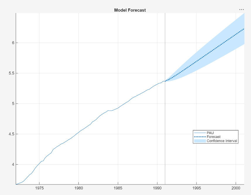
In the right pane, in the For(ARIMA_PAU) tab, is a plot containing the following time series:

• The time series data (blue line)

• Each h-step-ahead forecast (blue dashed line)

• The pointwise 95% Wald-based forecast intervals (blue region)

Compare the MMSE forecasts and forecasts based on 1000 simulated paths from the model into the forecast horizon.

1. In the Models pane, select the ARIMA_PAU model.

2. On the Modeler tab, in the Forecast section, click Forecast.

3. In the Forecast Model Response dialog box:

   1. Set Number of periods in forecast horizon to 40.

   2. Set Method > Simulation.

   3. Set Number of simulated paths to 1000.

   4. Click Forecast.

   

In the Forecasts pane, a variable FOR_ARIMA_PAU_2 appears. This variable is a structure array with the following fields:

• Forecast — fh-by-1 vector of pointwise means of the forecasted paths, with rows corresponding to the fh specified periods in the forecast horizon

• UpperConfidenceBound — fh-by-1 vector of upper confidence bounds of the pointwise 95% percentile-based forecast intervals

• LowerConfidenceBound — fh-by-1 vector of lower confidence bounds of the pointwise 95% percentile-based forecast intervals

In the right pane, in the For(ARIMA_PAU)_2 tab, is a plot containing the following time series:

• The time series data (blue line)

• The pointwise means of the simulated, h-step-ahead forecasted paths (blue dashed line)

• The pointwise 95% percentile-based forecast intervals (blue region)

The simulation-based and MMSE forecasts are similar.

Forecast the Stationary Model

Take the first difference of the log quarterly Australian CPI time series. In the Time Series pane, select the PAU time series. Then, on the Modeler tab, in the Transforms section, click Difference.

The differenced series is PAU_Diff. A plot of the series is, on the right pane, in the Plot(PAU_Diff) tab.

Fit an AR(2) model containing a constant to the differenced series.

1. In the Time Series pane, select PAU_Diff.

2. In the Modeler tab, in the Models section, click AR.

3. In the AR Model Parameters dialog box, set Autoregressive Order (p) to 2.

4. Click Estimate.

An estimation summary appears in the Fit(AR_PAU_Diff) tab, and the estimated model AR_PAU_Diff appears in the Models pane.

Generate MMSE forecasts into a 10-year horizon from the stationary model.

1. In the Models pane, select the ARIMA_PAU_Diff model.

2. On the Modeler tab, in the Forecast section, click Forecast.

3. In the Forecast Model Response dialog box, set Number of periods in forecast horizon to 40. Click Forecast.

In the Forecasts pane, a variable FOR_ARIMA_PAU_Diff appears. In the right pane, in the For(ARIMA_PAU_Diff) tab, is a plot containing the data, forecasts, and confidence intervals.

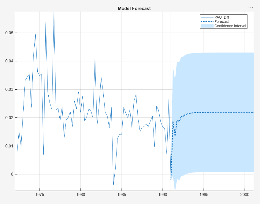
In the next 10 years, the Australian CPI rate is expected to settle at slightly above 2%, with a 95% confidence interval of about [0%, 4%].