predict

R2026b

Predict responses for new observations from panel data regression model

Since R2026b

Syntax

ypred = predict(EstMdl,X)

ypred = predict(EstMdl,X,groups)

[ypred,YPredCI] = predict(___)

[ypred,YPredCI] = predict(___,Name=Value)

Description

ypred = predict(EstMdl,X) returns the unconditional predicted responses ypred resulting from evaluating the estimated panel data regression model EstMdl at X, the observations of the predictor data in long format. X is an m-by-p matrix of predictor data, where m is the number of observations (for example, m = Tn for a balanced panel data set, where T is the number of measurement times and n is the number of subjects in the sample). Each row is an observation (all measurements) associated with a particular subject at a particular time, neither of which are known, and each column is a predictor variable.

ypred = predict(EstMdl,X,groups) specifies the group (subject-specific) identifiers groups associated with the observations for the unobserved effects in the estimated panel data regression model. Consequently, predict returns conditional predicted responses given the subject of each observation.

[ypred,YPredCI] = predict(___) additionally returns 95% prediction intervals for the predicted responses using any of the input argument combinations in the previous syntaxes.

[ypred,YPredCI] = predict(___,Name=Value) specifies additional options for the prediction intervals using one or more name-value arguments. For example, Confidence=0.9 computes 90% prediction intervals for the predicted responses.

Examples

Predict In-Sample Unconditional Responses from Fitted Panel Regression Model

Predict unconditional responses from a fitted random-effects panel data regression model using the default options. The data is in wide format, a 3-D array in which sample times are along the rows, predictors are along the columns, and subjects are along the pages.

Load the simulated, balanced panel data set Data_SimulatedBalancedPanel.mat, which is available when you open the live script for this example. The data set contains 12 microeconomic measurements of 1000 randomly selected people taken yearly from 2006 through 2020. The response variable in the model is a series of log wages, while all other variables in the data are predictors.

load Data_SimulatedBalancedPanel

For details on the data set, enter Description at the command line.

The variable Data is a 3-D numeric array containing the predictor and response variables. Each row is a time point in the sampling period, each column is a subject in the sample, and each page is a variable. The final variable in Data is the response variable (log wage series), while all other variables are predictors.

Create separate variables for the predictor and response data.

X = Data(:,:,1:(end-1));
Y = Data(:,:,end);

X is a 15-by-1000-by-11 numeric array of predictor data, and Y is a 15-by-1000 numeric matrix. For example, X(10,501,3) is the education level of subject 501 in 2015.

Create a binary numeric variable for whether the subject is female (coded as 1) by using predictor 2, and a binary numeric variable for whether the subject is married (coded as 1) by using predictor 9.

X(:,:,2) = double(X(:,:,2) == 1);
X(:,:,9) = double(X(:,:,9) == 1);

Assume that the heterogeneity is not associated with the predictor variables. Fit a random-effects panel data regression model to the data using he default options.

EstMdl = fitrepanel(X,Y);

Panel data information: 
Number of cross-sectional units (N):  1000
Number of periods (T):  15
Number of observations:  15000
Method of estimation:  random effects (GLS)

                     | Estimator    SE      tStat   pValue 
-----------------------------------------------------------
 x1                  |   0.0485   0.0003  154.4327   0     
 x2                  |  -0.3381   0.0324  -10.4265  0.0000 
 x3                  |   0.1003   0.0036   28.0246  0.0000 
 x4                  |  -0.1370   0.0389   -3.5231  0.0004 
 x5                  |  -0.0620   0.0047  -13.1530  0.0000 
 x6                  |   0.0087   0.0053    1.6637  0.0962 
 x7                  |  -0.0390   0.0112   -3.4902  0.0005 
 x8                  |  -0.0191   0.0071   -2.6853  0.0072 
 x9                  |  -0.0516   0.0107   -4.8406  0.0000 
 x10                 |   0.0741   0.0051   14.6575  0.0000 
 x11                 |   0.0016   0.0003    5.7319  0.0000 
 DisturbanceVariance |   0.0302                            
 EffectVariance      |   0.0947                            

EstMdl is a PanelModel object representing a fitted random-effects panel regression model.

The predict function accepts only numeric data in long format. Randomly select 25 observations from the predictor data, from which to predict responses, and randomly select 25 observations from the response data, from which to compare the predictions. Then, stack the observations.

rng(1,"twister")
[T,n,p] = size(X);
npred = 25;
rowIdx = randi(T,npred,1);
colIdx = randi(n,npred,1);

XPred = zeros(npred,p); % Preallocate data
yObs = zeros(npred,1);

for k = 1:npred
    XPred(k,:) = squeeze(X(rowIdx(k),colIdx(k),:)).';
    yObs(k) = Y(rowIdx(k),colIdx(k));
end

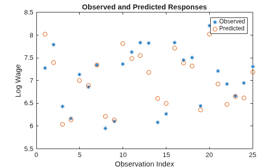
Predict responses for each selected observation from the predictor data. The format of the predictor data to use for prediction obscures the subject assignment, and no other inputs inform the subjects. Therefore, the resulting responses are unconditional. Compare the predictions and their observed values.

yPred = predict(EstMdl,XPred);

xp = (1:npred)';
plot(xp,yObs,"*",xp,yPred,"o")
xlabel("Observation Index")
ylabel("Log Wage")
title("Observed and Predicted Responses")
legend("Observed","Predicted")

mse = mean((yObs - yPred).^2)

mse = 
0.1007

The predicted responses are close to the corresponding observations, and the MSE is low.

Predict Out-of-Sample Conditional Responses from Fitted Panel Regression Model

Predict out-of-sample conditional responses from a fitted, one-way, fixed-effects panel data regression model using the default options. The data is in long format, a matrix in which each row is a measurement from a subject and a variable identifies the subjects.

Load the simulated, balanced panel data set Data_SimulatedBalancedPanel.mat, which is available when you open the live script for this example. The data set contains 12 microeconomic measurements of 1000 randomly selected people taken yearly from 2006 through 2020. The response variable in the model is a series of log wages, while all other variables in the data are predictors.

load Data_SimulatedBalancedPanel

For details on the data set, enter Description at the command line.

The variable DataTimeTable is a timetable containing the data. LogWage is the response variable, Group is the subject ID (grouping) variable, and all other variables are predictors. Each row is an observation for a subject at a time point in the sampling period (in other words, this data format is long).

Create a new timetable TT containing a binary numeric variable for whether the subject is female by using Gender, and a binary numeric variable for whether the subject is married by using MaritalStatus. Then, remove the corresponding variables from TT.

TT = DataTimeTable;
TT.IsFemale = double(TT.Gender == "female");
TT = movevars(TT,"IsFemale","Before","Gender");
TT.Gender = [];
TT.IsMarried = double(TT.MaritalStatus == "married");
TT = movevars(TT,"IsMarried","Before","MaritalStatus");
TT.MaritalStatus = [];

Suppose the estimation sample contains the observations from 2006 through 2015, and the holdout sample contains the observations from 2016 through 2020.

Create the estimation and holdout samples.

esttr = timerange("2006-01-01","2015-12-31");
hotr = timerange("2016-01-01","2020-12-31");
EstTT = TT(esttr,:);
HOTT = TT(hotr,:);

Fit a fixed-effects panel data regression model of the log wage series (LogWage) to all other variables, except the subject ID (Group), in the timetable. Specify the predictor and grouping variable names. fitfepanel assumes that the final variable is the response variable.

prednames = TT.Properties.VariableNames(1:end-2);
EstMdl = fitfepanel(EstTT,PredictorVariables=prednames,GroupVariable="Group");

Panel data information: 
Number of cross-sectional units (N):  1000
Number of periods (T):  10
Number of observations:  10000
Method of estimation:  fixed effects (within estimator)

                 | Estimator    SE     tStat   pValue 
------------------------------------------------------
 WorkExperience  |   0.0481   0.0006  77.6925   0     
 IsFemale        |    0        0                      
 Education       |    0        0                      
 Ethnicity       |    0        0                      
 IsBlueCollar    |  -0.0629   0.0068  -9.1928  0.0000 
 IsManufacturing |   0.0142   0.0078   1.8129  0.0698 
 IsSouth         |  -0.0254   0.0192  -1.3240  0.1855 
 IsCity          |  -0.0259   0.0111  -2.3353  0.0195 
 IsMarried       |  -0.0662   0.0170  -3.8933  0.0001 
 IsUnion         |   0.0746   0.0074  10.1137  0.0000 
 WeeksWorked     |   0.0017   0.0003   4.9530  0.0000 
 variance        |   0.0304                           

EstMdl is a PanelModel object representing a fitted, one-way, fixed-effects panel regression model.

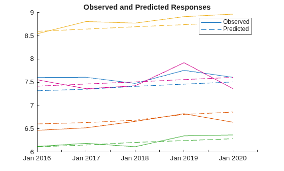
The predict function accepts numeric data only in long format. Supply the predictor observations and subject IDs in HOTT as numeric arrays. Predict a conditional response for each observation in the holdout sample. Include the prediction variable in the holdout sample timetable to align the prediction with other variables.

yPred = predict(EstMdl,HOTT{:,prednames},HOTT.Group);
HOTT.YPred = yPred;

yPred is a 5000-by-1 numeric vector of predicted log wages of all subjects from 2016 through 2020. Because predict has knowledge of the subject of each observation, the predictions are conditional on the subject.

Plot the predictions for a random selection of five subjects.

rng(1,"twister")
grp = randsample(1:1000,5,false);
t = HOTT.Time;
yObs = HOTT.LogWage;

figure
hold on
for j = 1:numel(grp)
    idx = HOTT.Group == grp(j);
    tmp1 = plot(t(idx),yObs(idx),"-");
    tmp2 = plot(t(idx),yPred(idx),"--");
    tmp2.Color = tmp1.Color;
end
hold off
title("Observed and Predicted Responses")
legend("Observed","Predicted")

Return 95% Prediction Intervals

Return the unconditional predicted responses and prediction intervals from the fitted random-effects panel data regression model in Predict In-Sample Unconditional Responses from Fitted Panel Regression Model. The data is in wide format.

Load and preprocess the data, fit the random-effects panel regression model, and randomly select 25 observations from which to generate predictions and prediction intervals.

load Data_SimulatedBalancedPanel
X = Data(:,:,1:(end-1));
Y = Data(:,:,end);
X(:,:,2) = double(X(:,:,2) == 1);
X(:,:,9) = double(X(:,:,9) == 1);
EstMdl = fitrepanel(X,Y);

Panel data information: 
Number of cross-sectional units (N):  1000
Number of periods (T):  15
Number of observations:  15000
Method of estimation:  random effects (GLS)

                     | Estimator    SE      tStat   pValue 
-----------------------------------------------------------
 x1                  |   0.0485   0.0003  154.4327   0     
 x2                  |  -0.3381   0.0324  -10.4265  0.0000 
 x3                  |   0.1003   0.0036   28.0246  0.0000 
 x4                  |  -0.1370   0.0389   -3.5231  0.0004 
 x5                  |  -0.0620   0.0047  -13.1530  0.0000 
 x6                  |   0.0087   0.0053    1.6637  0.0962 
 x7                  |  -0.0390   0.0112   -3.4902  0.0005 
 x8                  |  -0.0191   0.0071   -2.6853  0.0072 
 x9                  |  -0.0516   0.0107   -4.8406  0.0000 
 x10                 |   0.0741   0.0051   14.6575  0.0000 
 x11                 |   0.0016   0.0003    5.7319  0.0000 
 DisturbanceVariance |   0.0302                            
 EffectVariance      |   0.0947                            

rng(1,"twister")
[T,n,p] = size(X);
npred = 25;
rowIdx = randi(T,npred,1);
colIdx = randi(n,npred,1);
XPred = zeros(npred,p); % Preallocate data
yObs = zeros(npred,1);
for k = 1:npred
    XPred(k,:) = squeeze(X(rowIdx(k),colIdx(k),:)).';
    yObs(k) = Y(rowIdx(k),colIdx(k));
end

Generate predicted responses and 95% prediction intervals for each selected observation from the predictor data by returning both output arguments. The format of the predictor data to use for prediction obscures the subject assignment, and no other inputs inform the subjects. Therefore, the resulting responses are unconditional. Plot the predictions and prediction intervals, and the corresponding observed values.

[yPred,YPI] = predict(EstMdl,XPred);

xp = (1:npred)';
figure
plot(xp,yObs,"*",xp,yPred,"o")
hold on
plot(xp,YPI,LineStyle="none")
text(xp,YPI(:,1),"$\underbrace{}$",Interpreter="latex",HorizontalAlignment="center")
text(xp,YPI(:,2),"$\overbrace{}$",Interpreter="latex",HorizontalAlignment="center")
xlabel("Observation Index")
ylabel("Log Wage")
title("Observed and Predicted Responses with Prediction Intervals")
legend("Observed","Predicted")

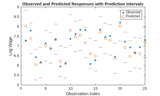
In the plot, the markers of the lower and upper bounds of the prediction intervals are braces. All observed values are within the respective 95% prediction intervals.

Return Predictions and Intervals for Average Responses

By default, predict returns prediction intervals for specific observations. This example shows how to specify predictions for the average response instead, using the fitted, one-way, fixed-effects panel data regression model in Predict Out-of-Sample Conditional Responses from Fitted Panel Regression Model.

Load and preprocess the data, and then fit the one-way, fixed-effects panel regression model.

load Data_SimulatedBalancedPanel
TT = DataTimeTable;
TT.IsFemale = double(TT.Gender == "female");
TT = movevars(TT,"IsFemale","Before","Gender");
TT.Gender = [];
TT.IsMarried = double(TT.MaritalStatus == "married");
TT = movevars(TT,"IsMarried","Before","MaritalStatus");
TT.MaritalStatus = [];

esttr = timerange("2006-01-01","2015-12-31");
hotr = timerange("2016-01-01","2020-12-31");
EstTT = TT(esttr,:);
HOTT = TT(hotr,:);

prednames = TT.Properties.VariableNames(1:end-2);
EstMdl = fitfepanel(EstTT,PredictorVariables=prednames,GroupVariable="Group");

Panel data information: 
Number of cross-sectional units (N):  1000
Number of periods (T):  10
Number of observations:  10000
Method of estimation:  fixed effects (within estimator)

                 | Estimator    SE     tStat   pValue 
------------------------------------------------------
 WorkExperience  |   0.0481   0.0006  77.6925   0     
 IsFemale        |    0        0                      
 Education       |    0        0                      
 Ethnicity       |    0        0                      
 IsBlueCollar    |  -0.0629   0.0068  -9.1928  0.0000 
 IsManufacturing |   0.0142   0.0078   1.8129  0.0698 
 IsSouth         |  -0.0254   0.0192  -1.3240  0.1855 
 IsCity          |  -0.0259   0.0111  -2.3353  0.0195 
 IsMarried       |  -0.0662   0.0170  -3.8933  0.0001 
 IsUnion         |   0.0746   0.0074  10.1137  0.0000 
 WeeksWorked     |   0.0017   0.0003   4.9530  0.0000 
 variance        |   0.0304                           

Generate conditional predictions for the average response, with a 90% prediction interval on the average, for each selected observation in the holdout sample by performing the following actions when you call predict:

• Specify the subject IDs.

• Specify Disturbance=false.

• Specify Confidence=0.90.

• Return both output arguments.

For three randomly selected holdout observations, plot the predictions and prediction intervals on the average response, and the corresponding observed values.

[yPred,YPI] = predict(EstMdl,HOTT{:,prednames},HOTT.Group,Disturbance=false, ...
    Confidence=0.90);
HOTT.YPred = yPred;
HOTT.YPI = YPI;

rng(1,"twister")
grp = randsample(1:1000,4,false);
t = HOTT.Time;
yObs = HOTT.LogWage;
figure
tiledlayout(2,2)
for j = 1:numel(grp)
    nexttile
    idx = HOTT.Group == grp(j);
    tmp1 = plot(t(idx),yObs(idx),"-");
    hold on
    tmp2 = plot(t(idx),yPred(idx),"o-");    
    tmp3 = plot(t(idx),YPI(idx,1),"--",t(idx),YPI(idx,2),"--");
    tmp3(2).Color = tmp3(1).Color;
    hold off
    title("Subject  = " + string(grp(j)))
end
legend("Observed","Predicted","Interval bounds",Location="southoutside")
sgtitle("Observed and Predicted Responses with 90% Intervals")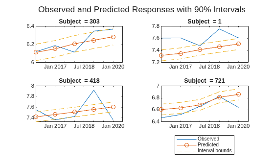

The prediction intervals are relative to the average response, so they are tighter than the prediction intervals for a specific response. Therefore, the observed response might be outside the interval more often than intervals for specific responses.

Predict Conditional Responses for New Subjects

Generate conditional predictions from random-effects and fixed-effects panel regression models on subjects not observed in the estimation data.

Consider the data generating process

$$y_{tj}=0.5x_{tj}+{\alpha }_j+0.1{\epsilon }_{tj}$$,

where $x_{tj}\sim N\left(0,1\right)$ is an iid set of predictor observations, $\alpha =\left[\begin{array}{ccc}2& 5& 8\end{array}\right]$, and ${\epsilon }_{tj}\sim N\left(0,0.1^2\right)$ is an iid series of disturbances.

Generate $T=5$ measurements for the $n=3$ subjects.

rng(1,"twister")
T = 5;
n = 3;
X = randn(T,n); 
alpha = [2 5 8]; 
y = 0.5*X + alpha + 0.1*randn(T,n);

Fit a random-effects model and a fixed-effects model to the simulated data.

EstMdlRE = fitrepanel(X,y);

Panel data information: 
Number of cross-sectional units (N):  3
Number of periods (T):  5
Number of observations:  15
Method of estimation:  random effects (GLS)

                     | Estimator    SE     tStat  pValue 
---------------------------------------------------------
 x1                  |   0.4021   0.0422  9.5178  0.0000 
 DisturbanceVariance |   0.0152                          
 EffectVariance      |   7.8880                          

EstMdlFE = fitfepanel(X,y);

Panel data information: 
Number of cross-sectional units (N):  3
Number of periods (T):  5
Number of observations:  15
Method of estimation:  fixed effects (within estimator)

          | Estimator    SE     tStat  pValue 
----------------------------------------------
 x1       |   0.4019   0.0418  9.6127  0.0000 
 variance |   0.0152                          

Predict the response for new random measurements on subject 2.

xnew2 = randn(1,1);
[ypredfe,ypife] = predict(EstMdlFE,xnew2,2); 
[ypredre,ypire] = predict(EstMdlRE,xnew2,2); 
fprintf('Known subject, random-effects model:  prediction = %.2f,  pred. interval = [%.2f, %.2f]\n',ypredre,ypire);

Known subject, random-effects model:  prediction = 5.54,  pred. interval = [5.25, 5.84]

fprintf('Known subject, fixed-effects model:   prediction = %.2f,  pred. interval = [%.2f, %.2f]\n',ypredfe,ypife);

Known subject, fixed-effects model:   prediction = 5.54,  pred. interval = [5.25, 5.83]

Conditional predictions generated from either model use the general formula $\underset{}{\overset{ˆ}{y_{t2}}}=x_{t2}\underset{}{\overset{ˆ}{\beta }}+\underset{}{\overset{ˆ}{{\alpha }_2}}$. The prediction variance uses a Bayesian estimate of the effects variance (conditioned on the subject).

Predict the response for new random measurements on a new subject with an ID of 4.

xnew4 = randn(1,1);
[ypredfenew,ypifenew] = predict(EstMdlFE,xnew4,4); 
[ypredrenew,ypirenew] = predict(EstMdlRE,xnew4,4); 
fprintf('New subject, random-effects model:  prediction = %.2f,  pred. interval = [%.2f, %.2f]\n',ypredrenew,ypirenew);

New subject, random-effects model:  prediction = 5.01,  pred. interval = [-1.37, 11.38]

fprintf('New subject, fixed-effects model:   prediction = %.2f,  pred. interval = [%.2f, %.2f]\n',ypredfenew,ypifenew);

New subject, fixed-effects model:   prediction = 5.01,  pred. interval = [-Inf, Inf]

Because subject 4 is not represented in the fitted models, the functions must compute unconditional predictions. For both models, the formula is $\underset{}{\overset{ˆ}{y_{t4}}}=x_{t4}\underset{}{\overset{ˆ}{\beta }}+\underset{}{\overset{‾}{\underset{}{\overset{ˆ}{\alpha }}}}$, where $\underset{}{\overset{‾}{\underset{}{\overset{ˆ}{\alpha }}}}$ is the mean of the estimated effects. For a random-effects model, the effects variance in the prediction variance formula derives from the estimation method, which is the within-transformation method, in this case. For the fixed-effects model, the prediction variance is infinite because the effects variance is infinite. Therefore, the interval is uninformative.

Input Arguments

EstMdl — Estimated panel data regression model

PanelModel object

Estimated panel data regression model, specified as a PanelModel object returned by fitfepanel or fitrepanel.

X — Predictor data X

numeric matrix

Predictor data X, specified as an m-by-p numeric matrix, where m is the total number of observations, and p is the number of predictor variables. X is in long format and the following conditions apply:

• Each row is an observation taken at a particular time from a particular subject, both of which are arbitrary. That is, row j contains the measurements for all predictors at time t for the subject g. If you specify the optional input groups, groups(j) is g.

• Column k contains the measurements of predictor variable k.

NaN values in X indicate missing measurements. predict computes predictions and prediction intervals using the raw input data and, therefore, outputs might contain NaNs as a result of missing input measurements.

Data Types: double

groups — Subject (group) identifiers

vector

Subject (group) identifiers for unobserved effects, specified as an m-by-1 vector of elements in EstMdl.GroupNames.

When you specify groups, predict returns conditional predicted responses given the specified subjects.

By default, predict returns unconditional predicted responses.

When groups contains subject IDs that are not in the fitted model EstMdl, predict ignores groups and returns unconditional predictions.

Data Types: double | categorical | cell | char | string

Name-Value Arguments

Specify optional pairs of arguments as Name1=Value1,...,NameN=ValueN, where Name is the argument name and Value is the corresponding value. Name-value arguments must appear after other arguments, but the order of the pairs does not matter.

Example: predict(EstMdl,X,Confidence=0.9) returns 90% prediction intervals for the predicted responses.

Confidence — Confidence level for prediction interval bounds

0.95 (default) | numeric scalar in [0,1]

Confidence level for the prediction interval bounds, specified as a numeric scalar in the interval [0,1].

For each input observation, a large number of randomly drawn prediction intervals covers the true response approximately 100*Confidence% of the time.

The default value is 0.95, which implies that the prediction interval bounds represent 95% prediction intervals.

Example: Confidence=0.9 specifies 90% prediction intervals.

Data Types: double

Disturbance — Flag to adjust prediction intervals by model disturbance variance

true (default) | false

Flag to the adjust prediction intervals by model disturbance variance, specified as true or false.

Value	Description
true	The variance of the predicted response at the arbitrary time t for subject j is $$\text{Var}({\widehat{y}}_{tj})=[\begin{array}{cc}1& x_{tj}\prime \end{array}]{\widehat{\Sigma }}_{\beta }\left[\begin{array}{c}1\\ x_{tj}\end{array}\right]+{\widehat{\sigma }}_{\alpha ,j}^2+{\widehat{\sigma }}_{\epsilon }^2.$$ The prediction intervals are for a particular response, given the predictor data.
false	The variance of the predicted response at the arbitrary time t for subject j is $$\text{Var}({\widehat{y}}_{tj})=[\begin{array}{cc}1& x_{tj}\prime \end{array}]{\widehat{\Sigma }}_{\beta }\left[\begin{array}{c}1\\ x_{tj}\end{array}\right]+{\widehat{\sigma }}_{\alpha ,j}^2.$$ The prediction intervals are for the average response, given the predictor data.

In the above description, note the following:

• [1 x_tj] is the vector of predictor measurements for an observation, with 1 corresponding to the overall effect (model intercept). x_tj are rows of the input predictor data X corresponding to the coefficients in EstMdl.Coefficients.

• $${\widehat{\Sigma }}_{\beta }$$ is the estimated covariance matrix of the coefficient estimates, with entries in the first row, first column corresponding to the covariances associated with the overall effect.

• $${\widehat{\sigma }}_{\alpha ,j}^2$$ is the estimated effects variance for subject j; its value depends on the type of panel regression model (EstMdl.Type) and the type of prediction, either conditional or unconditional:

  • EstMdl.EffectVariance, for unconditional prediction or for predictions on new subjects

  • Bayesian estimate of the effect variance, for conditional predictions of known subjects

  For more details, see fitrepanel or fitfepanel.

• $${\widehat{\sigma }}_{\epsilon }^2$$ is the estimated disturbance variance.

• For unconditional prediction, subject information is not available and predictions target an arbitrary subject. Therefore, you can remove indices j from the equations.

Example: Disturbance=false

Data Types: logical

Output Arguments

ypred — Predicted responses

numeric vector

Predicted responses, returned as an m-by-1 numeric vector.

When you specify groups, predict returns conditional predicted responses given the specified subjects. Otherwise, predict returns unconditional predicted responses.

YPredCI — Wald-type prediction intervals

numeric matrix

Wald-type prediction intervals, returned as an m-by-2 numeric matrix. YPredCI(j,:) = [lower upper] is the 100*Confidence% prediction interval of predicted response j, where lower is the lower bound and upper is the upper bound of the interval.

When you specify groups, predict returns prediction intervals conditional on the specified subjects. Otherwise, predict returns unconditional prediction intervals.

When EstMdl.Type is "FixedEffects" and ypred contains unconditional predictions (that is,you do not specify groups), predict returns uninformative prediction intervals for all input observations [-Inf,Inf].

More About

Unconditional Prediction

An unconditional prediction from a panel regression model is the response $$\widehat{y}$$ resulting from evaluating the model at given predictor measurements, and assuming heterogeneity is 0 and an overall intercept is appropriate.

Symbolically, the unconditional prediction at the arbitrary time t for the arbitrary subject k is

$${\widehat{y}}_{jk}=x_{jk}\widehat{\beta }+\widehat{\alpha },$$

where:

• x_jk contains the given predictor measurements.

• $$\widehat{\beta }$$ is the vector of estimated regression coefficients without an intercept.

• $$\widehat{\alpha }$$ is the estimated intercept.

Conditional Prediction

A conditional prediction from a panel regression model is the response $$\widehat{y}$$ resulting from evaluating the model at given predictor measurements and using the estimated effect for the given subject. In other words, the distribution of the prediction is conditioned on the predictor data and subject.

Symbolically, the conditional prediction at the arbitrary time t for the subject g_k is

$${\widehat{y}}_{jk}=x_{jk}\widehat{\beta }+{\widehat{\alpha }}_k,$$

where:

• x_jk contains the given predictor measurements.

• $$\widehat{\beta }$$ is the vector of estimated regression coefficients without an intercept.

• $${\widehat{\alpha }}_k$$ is the estimated effect of subject g_k.

Panel Data

A panel data set contains the measurements of n subjects measured at most T times over a sampling time frame. Panel data is a type of longitudinal data resulting from an observational study, rather than a controlled experiment. This distinction affects regression procedures used to analyze these types of data sets. (To analyze longitudinal data, see fitlme, fitlmematrix, and fitrm.)

You can format panel data sets in wide format or long format. In the following discussion, an observation is all measurements (predictors x_i, i = 1,…,p and response y data) of a subject (g_k, k = 1,...,n) at a particular time (t_j, j = 1,…,T).

In wide format, the predictor data set X (input X) is a T-by-n-by-p 3-D numeric array, where rows correspond to contemporaneous sampling times in increasing order by row, columns correspond to individual subjects, and pages correspond to predictor variables. The response data set Y (input Y) in wide format is a T-by-n matrix. The figure below illustrates the predictor and response data in wide format.

For a data set in this format, you can clearly infer the sampling time and subject by the corresponding row and column, respectively. An observation of subject g_k at time t_j is the set {X(j,k,:), Y(j,k)}. For example, the boxed values in the figure comprise the observation of subject g₂ at time t₁.

In long format, the predictor data set X is an m-by-p matrix, where $$m={\displaystyle \sum _{j=1}^n{T}_j},$$ the total sample size. Each row contains all predictor measurements of a particular subject at a particular time, and each column is a predictor variable. The response data set y is an m-by-1 vector, where each row is the response of the corresponding subject at the corresponding time. For data in this format, you cannot infer the subject and sampling time to which each observation belongs. A variable of subject identifiers (group variable), an m-by-1 vector, is required. For each subject, observations are recorded in increasing order by row. The figure below illustrates the predictor and response data in long format.

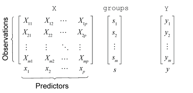
Row j of the subject identifier vector s_j is in the set {g₁,g₂,…,g_n}. This figure illustrates the variables for all observations of subject g₂ (s = g₂, coded as g2). In the figure, t_j = t(j). Because only those observations belonging to subject g ₂ are displayed, the row indices are not clear, but the sampling times are clear and, therefore, labeled.

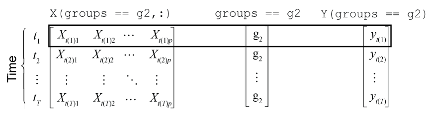
An observation of subject g_k at time t_j is the set {Xgk(j,:), Ygk(j)}, where Xgk = X(groups == gk,:) and Ygk = Y(groups == gk). For example, the boxed values in the figure comprise the observation of subject g₂ at time t₁.

A panel data set in a table or timetable is in long format. The Time variable of a timetable specifies the sampling times of the observations.

Regardless of format, when the data set contains the measurements for all subjects and sampling times, the data set is balanced. Otherwise, the data set is unbalanced.

Version History

Introduced in R2026b