particleoptions

Sequential Monte Carlo sampler options

Since R2026a

Description

When you analyze a Bayesian nonlinear non-Gaussian state-space model (bnlssm model object), particleoptions enables you to specify common sequential Monte Carlo (SMC) sampler specifications through all stages of your workflow.

Creation

Syntax

options = particleoptions

options = particleoptions(Property=Value)

Description

options = particleoptions creates an SMC sampler particle options object with default options that specify how to treat particles while drawing samples from the posterior distribution of a Bayesian nonlinear state-space model (bnlssm model object).

options = particleoptions(Property=Value) sets properties using name-value arguments. For example, particleoptions(NumParticles=1e4,NewSamples="auxiliary") specifies drawing 10,000 particles per sample time point from the proposal distribution and to use the auxiliary SMC sampler.

Properties

NumParticles — Number of particles

1000 (default) | positive integer

Number of particles for SMC, specified as a positive integer.

Example: NumParticles=1e4

Data Types: double

NewSamples — SMC proposal distribution

"bootstrap" (default) | "auxiliary" | "optimal" | "unscented" | character vector

Since R2025a

SMC proposal (importance) distribution, specified as a value in this table.

Value	SMC Sampler	Description
"auxiliary" (since R2026a)	Auxiliary filter [6]	SMC samples particles by using a reweight-resample strategy, which uses local approximations of the nonlinear state-space model and is informed by the observations. This option is available only for models with observation noise (nonzero D).
"bootstrap"	Bootstrap forward filter [4]	SMC samples particles form the state transition distribution (observations do not inform the sampler). This option is available only for models with observation noise (nonzero D). This method has a relatively low computational cost, but it does not inform the routine of the current observations, which can increase the Monte Carlo sampling variance.
"optimal"	Conditionally optimal proposal [2]	SMC samples particles from the one-step filtering distribution with incremental weights proportional to the likelihood (observations inform the sampler). The weights have minimum variance. This option is available for the following tractable models supplied in equation form: Nonlinear state transition equation and a linear measurement equation Nonlinear model with deterministic state transition equation (B = 0)
"unscented"	Unscented transformation [7]	SMC proposal distribution is the one-step filtering distribution approximated by the unscented transformation (observations inform the sampler). This option is available only for models in equation form with observation noise (nonzero D). By default, this option uses the filtered state mean as the representative point, around which the algorithm generates sigma points. To specify all particles as representative points for the unscented transformation, set MultiPassUnscented=true. This setting provides a higher-quality proposal, but it is more computationally expensive.

Example: NewSamples="unscented"

Data Types: char | string

Resample — SMC resampling method

"multinomial" (default) | "residual" | "systematic"

SMC resampling method, specified as a value in this table.

Value	Description
"multinomial"	At time t, the set of previously generated particles (parent set) follows a standard multinomial distribution, with probabilities proportional to their weights. An offspring set is resampled with replacement from the parent set [1].
"residual"	Residual sampling, a modified version of multinomial resampling that can produce an estimator with lower variance than the multinomial resampling method [5].
"systematic"	Systematic sampling, which produces an estimator with lower variance than the multinomial resampling method [3].

Resampling methods downsample insignificant particles to achieve a smaller estimator variance than if no resampling is performed and to avoid sampling from a degenerate proposal [3].

Example: Resample="residual"

Data Types: char | string

Cutoff — Effective sample size threshold for resampling

0.5*NumParticles (default) | nonnegative scalar

Effective sample size threshold, below which particleoptions resamples particles, specified as a nonnegative scalar. For more details, see [3], Ch. 12.3.3.

Tip

• To resample during every period, set Cutoff=numparticles, where numparticles is the value of the NumParticles name-value argument.

• To avoid resampling, set Cutoff=0.

Example: Cutoff=0.75*numparticles

Data Types: double

Examples

Default Particle Options Object

Create a default particle options object, and then adjust the default particle sampler and number of sampled particles. Then, pass it to a Bayesian nonlinear state-space model and fit the model to simulated data.

Consider this Bayesian nonlinear state-space model in equation.

$$\begin{array}{l}{x}_t=\varphi x_{t-1}+\sigma u_t\\ y_t\sim Poisson(\lambda e^{x_t}),\end{array}$$

where the parameters in $\Theta =\left\{\varphi ,\sigma ,\lambda \right\}$ have the following priors:

• $\varphi \sim N_{\left(-1,1\right)}\left(m_0,v_0^2\right)$, that is, a truncated normal distribution with $\varphi \in \left[-1,1\right]$.

• ${\sigma }^2\sim IG\left(a_0,b_0\right)$, that is, an inverse gamma distribution with shape $a_0$ and scale $b_0$.

• $\lambda \sim Gamma\left({\alpha }_0,{\beta }_0\right)$, that is, a gamma distribution with shape ${\alpha }_0$ and scale ${\beta }_0$.

Simulate Series

Consider this data-generating process (DGP).

$$\begin{array}{l}{x}_t=0.7x_{t-1}+\sqrt{0.2}{u}_t\\ y_t\sim Poisson(3e^{x_t}),\end{array}$$

where the series $u_t$ is a standard Gaussian series of random variables.

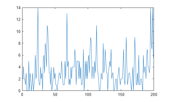
Simulate a series of 200 observations from the process.

rng(1,"twister")    % For reproducibility
T = 200;
thetaDGP = [0.7; 0.2; 3];

numparams = numel(thetaDGP);

MdlXSim = arima(AR=thetaDGP(1),Variance=thetaDGP(2), ...
    Constant=0);
xsim = simulate(MdlXSim,T);
y = random("poisson",thetaDGP(3)*exp(xsim));

figure
plot(y)

Create and Adjust Default Particle Options Object

Create and display the default SMC particle sampler options by calling particleoptions without setting any inputs.

options = particleoptions;
options

options = 
  particleoptions with properties:

    NumParticles: 1000
      NewSamples: "bootstrap"
        Resample: "multinomial"
          Cutoff: 500

options is a particleoptions object containing properties that specify particle sampling specifications for the SMC sampler.

Specify use of the auxiliary algorithm for sampling particles during SMC by setting the NewSamples property of options using dot notation.

options.NewSamples = "auxiliary";

Create Bayesian Nonlinear Prior Model

A prior distribution is required to compose a posterior distribution. The Local Functions section contains the functions paramMap and priorDistribution required to specify the Bayesian nonlinear state-space model. The paramMap function specifies the state-space model structure and initial state moments. The priorDistribution function returns the log of the joint prior distribution of the state-space model parameters. You can use the functions only within this script.

Create a Bayesian nonlinear state-space model for the DGP.

• Arbitrarily choose values for the hyperparameters.

• Indicate that the state-space model observation equation is expressed as a distribution.

• To speed up computations, the arguments A and LogY of the paramMap function are written to enable simultaneous evaluation of the transition and observation densities of multiple particles. Specify this characteristic by using the Multipoint name-value argument.

• Specify the SMC particle sampler options options.

% pi(phi,sigma2) hyperparameters
m0 = 0;                 
v02 = 1;
a0 = 1;
b0 = 1;

% pi(lambda) hyperparameters
alpha0 = 3;
beta0 = 1;

hyperparams = [m0 v02 a0 b0 alpha0 beta0];

PriorMdl = bnlssm(@paramMap,@(x)priorDistribution(x,hyperparams), ...
    ObservationForm="distribution",Multipoint=["A" "LogY"],ParticleOptions=options);

PriorMdl is a bnlssm model specifying the state-space model structure and prior distribution of the state-space model parameters. Because PriorMdl contains unknown values, it serves as a template for posterior estimation with observations.

Choose Initial Parameter Values

Arbitrarily choose a set of initial parameter for the MCMC sampler.

theta0 = [0.5; 0.1; 2]; 

Estimate Posterior

Estimate the posterior by passing the prior model, simulated data, and initial parameter values to estimate.

PosteriorMdl = estimate(PriorMdl,y,theta0);

         Optimization and Tuning        
      | Params0  Optimized  ProposalStd 
----------------------------------------
 c(1) |  0.5000    0.6001      0.0979   
 c(2) |  0.1000    0.2166      0.0413   
 c(3) |   2        2.8669      0.2828   
 
     Posterior Distributions of Parameters     
      |  Mean     Std   Quantile05  Quantile95 
-----------------------------------------------
 c(1) | 0.5951  0.0974    0.4193      0.7453   
 c(2) | 0.2522  0.0545    0.1690      0.3502   
 c(3) | 2.8667  0.2700    2.4043      3.2990   

    Posterior Distributions of Final States    
      |  Mean     Std   Quantile05  Quantile95 
-----------------------------------------------
 x(1) | 0.4568  0.3541    -0.1100     1.0224   
Proposal acceptance rate = 47.50%

PosteriorMdl.ParamMap

ans = function_handle with value:
    @paramMap

ThetaPostDraws = PosteriorMdl.ParamDistribution;
[numParams,numDraws] = size(ThetaPostDraws)

numParams = 
3

numDraws = 
1000

estimate finds an optimal proposal distribution for the MCMC sampler by using the tune function, and prints the optimal moments to the command line. estimate also displays a summary of the posterior distribution of the parameters. The true values of the parameters are close to their corresponding posterior means; all are within their corresponding 95% credible intervals.

PosteriorMdl is a bnlssm object representing the posterior distribution.

• PosteriorMdl.ParamMap is the function handle to the function representing the state-space model structure; it is the same function as PrioirMdl.ParamMap.

• ThetaPostDraws is a 3-by-1000 matrix of draws from the posterior distribution. By default, estimate treats the first 100 draws as a burn-in sample and excludes them from the results.

To diagnose the MCMC sampler, create trace plots of the posterior parameter draws.

paramnames = ["\phi" "\sigma^2" "\lambda"];

figure
h = tiledlayout(3,1);
for j = 1:numParams
    nexttile
    plot(ThetaPostDraws(j,:))
    hold on
    yline(thetaDGP(j))
    ylabel(paramnames(j))
end
title(h,"Posterior Trace Plots")

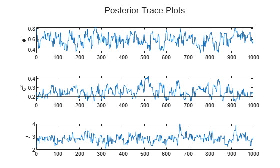
The sampler eventually settles at near the true values of the parameters. In this case, the sample shows serial correlation and transient behavior. You can remedy serial correlation in the sample by adjusting the Thin name-value argument, and you can remedy transient effects by increasing the burn-in period using the BurnIn name-value argument.

Local Functions

These functions specify the state-space model parameter mappings, in distribution form, and the log prior distribution of the parameters.

function [A,B,LogY,Mean0,Cov0,StateType] = paramMap(theta)
A = theta(1); 
B = sqrt(theta(2));
LogY = @(y,x)y.*(x + log(theta(3)))- exp(x).*theta(3);
Mean0 = 0;
Cov0 = 2;
StateType = 0;     % Stationary state process
end

function logprior = priorDistribution(theta,hyperparams)
% Prior of phi
m0 = hyperparams(1);
v20 = hyperparams(2);
pphi = makedist("normal",mu=m0,sigma=sqrt(v20));
pphi = truncate(pphi,-1,1);
lpphi = log(pdf(pphi,theta(1)));

% Prior of sigma2
a0 = hyperparams(3);
b0 = hyperparams(4);
lpsigma2 = -a0*log(b0) - log(gamma(a0)) + (-a0-1)*log(theta(2)) - ...
    1./(b0*theta(2));

% Prior of lambda
alpha0 = hyperparams(5);
beta0 = hyperparams(6);
plambda = makedist("gamma",alpha0,beta0);
lplambda = log(pdf(plambda,theta(3))); 

logprior = lpphi + lpsigma2 + lplambda;
end

Specify Particle Sampler Options for SMC

Specify particle sampler options for all SMC implementations of a Bayesian nonlinear state-space model.

Consider this Bayesian nonlinear state-space model and DGP in Default Particle Options Object.

Simulate a series of responses from the DGP.

rng(1,"twister")    % For reproducibility
T = 200;
thetaDGP = [0.7; 0.2; 3];

numparams = numel(thetaDGP);

MdlXSim = arima(AR=thetaDGP(1),Variance=thetaDGP(2), ...
    Constant=0);
xsim = simulate(MdlXSim,T);
y = random("poisson",thetaDGP(3)*exp(xsim));

Specify the following SMC particle sampler options:

• The auxiliary algorithm for sampling particles

• Sample 2,000 particles per time point

• Residual particle resample method

options = particleoptions(NewSamples="auxiliary",Resample="residual");

Create a Bayesian nonlinear state-space prior model. Specify the SMC particle sampler options.

% pi(phi,sigma2) hyperparameters
m0 = 0;                 
v02 = 1;
a0 = 1;
b0 = 1;

% pi(lambda) hyperparameters
alpha0 = 3;
beta0 = 1;

hyperparams = [m0 v02 a0 b0 alpha0 beta0];

PriorMdl = bnlssm(@paramMap,@(x)priorDistribution(x,hyperparams), ...
    ObservationForm="distribution",Multipoint=["A" "LogY"],ParticleOptions=options); 

Estimate the posterior by passing the prior model, simulated data, and initial parameter values to estimate.

theta0 = [0.5; 0.1; 2];
[PosteriorMdl,estParams] = estimate(PriorMdl,y,theta0);

         Optimization and Tuning        
      | Params0  Optimized  ProposalStd 
----------------------------------------
 c(1) |  0.5000    0.6989      0.0756   
 c(2) |  0.1000    0.1999      0.0544   
 c(3) |   2        2.9738      0.2521   
 
     Posterior Distributions of Parameters     
      |  Mean     Std   Quantile05  Quantile95 
-----------------------------------------------
 c(1) | 0.5888  0.0970    0.4277      0.7494   
 c(2) | 0.2420  0.0489    0.1746      0.3325   
 c(3) | 2.8837  0.2812    2.3529      3.3596   

    Posterior Distributions of Final States    
      |  Mean     Std   Quantile05  Quantile95 
-----------------------------------------------
 x(1) | 0.4796  0.3550    -0.1100     1.0591   
Proposal acceptance rate = 35.40%

PosteriorMdl.ParticleOptions

ans = 
  particleoptions with properties:

    NumParticles: 1000
      NewSamples: "auxiliary"
        Resample: "residual"
          Cutoff: 500

estimate uses the particle sampler options in PriorMdl.ParticleOptions when it implements SMC.

Estimate smoothed state values from the posterior distribution.

states = smooth(PosteriorMdl,y,estParams,Method="marginal");

smooth implements SMC to estimate states; it uses the options in PosteriorMdl.ParticleOptions to sample particles.

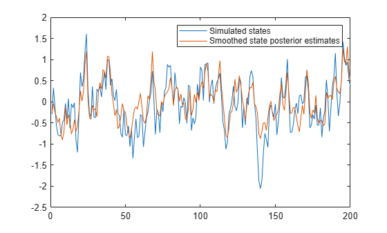
Visually compare the simulated states and smoothed state posterior estimates.

figure
plot([xsim states])
legend(["Simulated states" "Smoothed state posterior estimates"])

Local Functions

These functions specify the state-space model parameter mappings, in distribution form, and the log prior distribution of the parameters.

function [A,B,LogY,Mean0,Cov0,StateType] = paramMap(theta)
A = theta(1); 
B = sqrt(theta(2));
LogY = @(y,x)y.*(x + log(theta(3)))- exp(x).*theta(3);
Mean0 = 0;
Cov0 = 2;
StateType = 0;     % Stationary state process
end

function logprior = priorDistribution(theta,hyperparams)
% Prior of phi
m0 = hyperparams(1);
v20 = hyperparams(2);
pphi = makedist("normal",mu=m0,sigma=sqrt(v20));
pphi = truncate(pphi,-1,1);
lpphi = log(pdf(pphi,theta(1)));

% Prior of sigma2
a0 = hyperparams(3);
b0 = hyperparams(4);
lpsigma2 = -a0*log(b0) - log(gamma(a0)) + (-a0-1)*log(theta(2)) - ...
    1./(b0*theta(2));

% Prior of lambda
alpha0 = hyperparams(5);
beta0 = hyperparams(6);
plambda = makedist("gamma",alpha0,beta0);
lplambda = log(pdf(plambda,theta(3))); 

logprior = lpphi + lpsigma2 + lplambda;
end

References

[1] Andrieu, Christophe, Arnaud Doucet, and Roman Holenstein. "Particle Markov Chain Monte Carlo Methods." Journal of the Royal Statistical Society Series B: Statistical Methodology 72 (June 2010): 269–342. https://doi.org/10.1111/j.1467-9868.2009.00736.x.

[2] Doucet, Arnaud, Simon Godsill, and Christophe Andrieu. "On Sequential Monte Carlo Sampling Methods for Bayesian Filtering." Statistics and Computing 10 (July 2000): 197–208. https://doi.org/10.1023/A:1008935410038.

[3] Durbin, J, and Siem Jan Koopman. Time Series Analysis by State Space Methods. 2nd ed. Oxford: Oxford University Press, 2012.

[4] Gordon, Neil J., David J. Salmond, and Adrian F. M. Smith. "Novel Approach to Nonlinear/Non-Gaussian Bayesian State Estimation." IEE Proceedings F Radar and Signal Processing 140 (April 1993): 107–113. https://doi.org/10.1049/ip-f-2.1993.0015.

[5] Liu, Jun, and Rong Chen. "Sequential Monte Carlo Methods for Dynamic Systems." Journal of the American Statistical Association 93 (September 1998): 1032–1044. https://dx.doi.org/10.1080/01621459.1998.10473765.

[6] Pitt, Michael K., and Neil Shephard. "Filtering via Simulation: Auxiliary Particle Filters." Journal of the American Statistical Association 94 (June 1999): 590–599. https://doi.org/10.1080/01621459.1999.10474153.

[7] van der Merwe, Rudolph, Arnaud Doucet, Nando de Freitas, and Eric Wan. "The Unscented Particle Filter." Advances in Neural Information Processing Systems 13 (November 2000). https://dl.acm.org/doi/10.5555/3008751.3008833.

Version History

Introduced in R2026a