Simulate Regression Models with ARMA Errors

Simulate an AR Error Model

This example shows how to simulate sample paths from a regression model with AR errors without specifying presample disturbances.

Specify the regression model with AR(2) errors:

$$\begin{array}{l}{y}_t=2+X_t\left[\begin{array}{l}-2\\ 1.5\end{array}\right]+u_t\\ u_t=0.75u_{t-1}-0.5u_{t-2}+{\epsilon }_t,\end{array}$$

where $${\epsilon }_t$$ is Gaussian with mean 0 and variance 1.

Beta = [-2; 1.5];
Intercept = 2;
a1 = 0.75;
a2 = -0.5;
Variance = 1;
Mdl = regARIMA('AR',{a1, a2},'Intercept',Intercept,...
    'Beta',Beta,'Variance',Variance);

Generate two length T = 50 predictor series by random selection from the standard Gaussian distribution.

T = 50;
rng(1); % For reproducibility
X = randn(T,2);

The software treats the predictors as nonstochastic series.

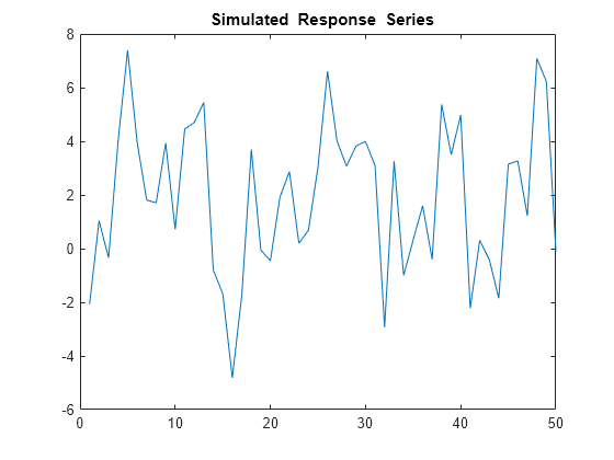
Generate and plot one sample path of responses from Mdl.

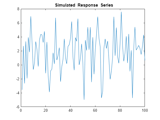
rng(2);
ySim = simulate(Mdl,T,'X',X);

figure
plot(ySim)
title('{\bf Simulated Response Series}')

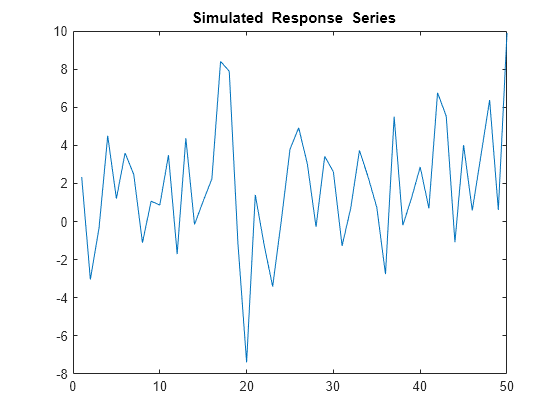
simulate requires P = 2 presample unconditional disturbances ($$u_t$$) to initialize the error series. Without them, as in this case, simulate sets the necessary presample unconditional disturbances to 0.

Alternatively, filter a random innovation series through Mdl using filter.

rng(2);
e = randn(T,1);
yFilter = filter(Mdl,e,'X',X);

figure
plot(yFilter)
title('{\bf Simulated Response Series Using Filtered Innovations}')

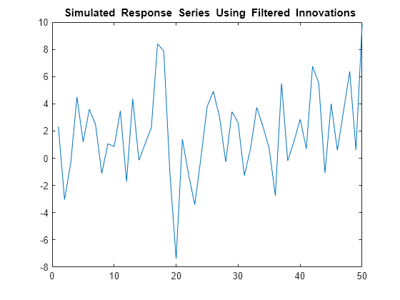
The plots suggest that the simulated responses and the responses generated from the filtered innovations are equivalent.

Simulate 1000 response paths from Mdl. Assess transient effects by plotting the unconditional disturbance (U) variances across the simulated paths at each period.

numPaths = 1000;
[Y,~,U] = simulate(Mdl,T,'NumPaths',numPaths,'X',X);

figure
h1 = plot(Y,'Color',[.85,.85,.85]);
title('{\bf 1000 Simulated Response Paths}')
hold on
h2 = plot(1:T,Intercept+X*Beta,'k--','LineWidth',2);
legend([h1(1),h2],'Simulated Path','Mean')
hold off

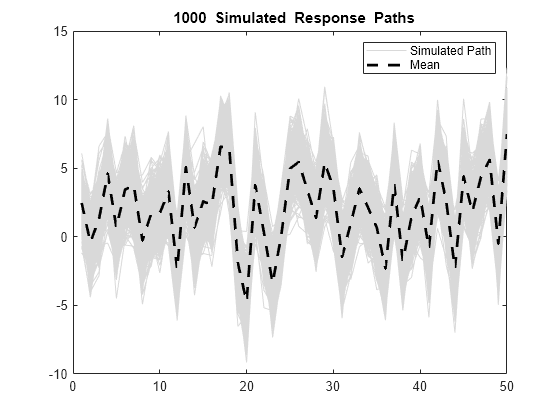
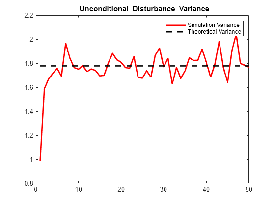
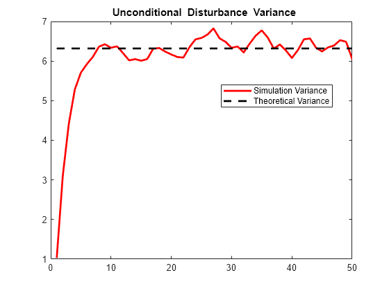
figure
h1 = plot(var(U,0,2),'r','LineWidth',2);
hold on
theoVarFix = ((1-a2)*Variance)/((1+a2)*((1-a2)^2-a1^2));
h2 = plot([1 T],[theoVarFix theoVarFix],'k--','LineWidth',2);
title('{\bf Unconditional Disturbance Variance}')
legend([h1,h2],'Simulation Variance','Theoretical Variance')
hold off

The simulated response paths follow their theoretical mean, $$c+X\beta$$, which is not constant over time (and might look nonstationary).

The variance of the process is not constant, but levels off at the theoretical variance by the 10th period. The theoretical variance of the AR(2) error model is

$$\frac{\left(1-a_2\right){\sigma }_{\epsilon }^2}{\left(1+a_2\right)\left[{\left(1-a_2\right)}^2-a_1^2\right]}=\frac{(1+0.5)}{(1-0.5)\left[{(1+0.5)}^2-{0.75}^2\right]}=1.78$$

You can reduce transient effects is by partitioning the simulated data into a burn-in portion and a portion for analysis. Do not use the burn-in portion for analysis. Include enough periods in the burn-in portion to overcome the transient effects.

burnIn = 1:10;
notBurnIn = burnIn(end)+1:T;
Y = Y(notBurnIn,:);
X = X(notBurnIn,:);
U = U(notBurnIn,:);
figure
h1 = plot(notBurnIn,Y,'Color',[.85,.85,.85]);
hold on
h2 = plot(notBurnIn,Intercept+X*Beta,'k--','LineWidth',2);
title('{\bf 1000 Simulated Response Paths for Analysis}')
legend([h1(1),h2],'Simulated Path','Mean')
hold off

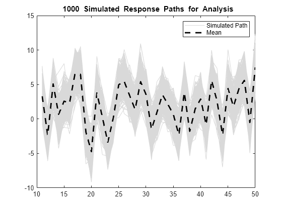
figure
h1 = plot(notBurnIn,var(U,0,2),'r','LineWidth',2);
hold on
h2 = plot([notBurnIn(1) notBurnIn(end)],...
    [theoVarFix theoVarFix],'k--','LineWidth',2);
title('{\bf Converged Unconditional Disturbance Variance}')
legend([h1,h2],'Simulation Variance','Theoretical Variance')
hold off

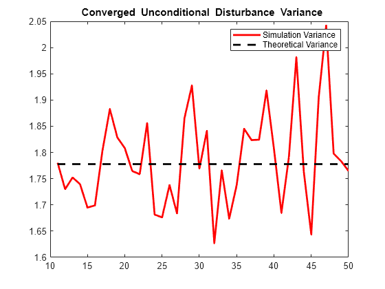
Unconditional disturbance simulation variances fluctuate around the theoretical variance due to Monte Carlo sampling error. Be aware that the exclusion of the burn-in sample from analysis reduces the effective sample size.

Simulate an MA Error Model

This example shows how to simulate responses from a regression model with MA errors without specifying a presample.

Specify the regression model with MA(8) errors:

$$\begin{array}{l}{y}_t=2+X_t\left[\begin{array}{l}-2\\ 1.5\end{array}\right]+u_t\\ u_t={\epsilon }_t+0.4{\epsilon }_{t-1}-0.3{\epsilon }_{t-4}+0.2{\epsilon }_{t-8},\end{array}$$

where $${\epsilon }_t$$ is Gaussian with mean 0 and variance 0.5.

Beta = [-2; 1.5];
Intercept = 2;
b1 = 0.4;
b4 = -0.3;
b8 = 0.2;
Variance = 0.5;
Mdl = regARIMA('MA',{b1, b4, b8},'MALags',[1 4 8],...
    'Intercept',Intercept,'Beta',Beta,'Variance',Variance);

Generate two length T = 100 predictor series by random selection from the standard Gaussian distribution.

T = 100;
rng(4); % For reproducibility
X = randn(T,2);

The software treats the predictors as nonstochastic series.

Generate and plot one sample path of responses from Mdl.

rng(5);
ySim = simulate(Mdl,T,'X',X);

figure
plot(ySim)
title('{\bf Simulated Response Series}')

simulate requires Q = 8 presample innovations ($${\epsilon }_t$$) to initialize the error series. Without them, as in this case, simulate sets the necessary presample innovations to 0.

Alternatively, use filter to filter a random innovation series through Mdl.

rng(5);
e = randn(T,1);
yFilter = filter(Mdl,e,'X',X);

figure
plot(yFilter)
title('{\bf Simulated Response Series Using Filtered Innovations}')

The plots suggest that the simulated responses and the responses generated from the filtered innovations are equivalent.

Simulate 1000 response paths from Mdl. Assess transient effects by plotting the unconditional disturbance (U) variances across the simulated paths at each period.

numPaths = 1000;
[Y,~,U] = simulate(Mdl,T,'NumPaths',numPaths,'X',X);

figure
h1 = plot(Y,'Color',[.85,.85,.85]);
title('{\bf 1000 Simulated Response Paths}')
hold on
h2 = plot(1:T,Intercept+X*Beta,'k--','LineWidth',2);
legend([h1(1),h2],'Simulated Path','Mean')
hold off

figure
h1 = plot(var(U,0,2),'r','LineWidth',2);
hold on
theoVarFix = (1+b1^2+b4^2+b8^2)*Variance;
h2 = plot([1 T],[theoVarFix theoVarFix],'k--','LineWidth',2);
title('{\bf Unconditional Disturbance Variance}')
legend([h1,h2],'Simulation Variance','Theoretical Variance')
hold off

The simulated paths follow their theoretical mean, $$c+X\beta$$, which is not constant over time (and might look nonstationary).

The variance of the process is not constant, but levels off at the theoretical variance by the 15th period. The theoretical variance of the MA(8) error model is

$$(1+b_1^2+b_4^2+b_8^2){\sigma }_{\epsilon }^2=\left(1+{0.4}^2+{(-0.3)}^2+{0.2}^2\right)0.5=0.645.$$

You can reduce transient effects is by partitioning the simulated data into a burn-in portion and a portion for analysis. Do not use the burn-in portion for analysis. Include enough periods in the burn-in portion to overcome the transient effects.

burnIn = 1:15;
notBurnIn = burnIn(end)+1:T;
Y = Y(notBurnIn,:);
X = X(notBurnIn,:);
U = U(notBurnIn,:);
figure
h1 = plot(notBurnIn,Y,'Color',[.85,.85,.85]);
hold on
h2 = plot(notBurnIn,Intercept+X*Beta,'k--','LineWidth',2);
title('{\bf 1000 Simulated Response Paths for Analysis}')
legend([h1(1),h2],'Simulated Path','Mean')
axis tight
hold off

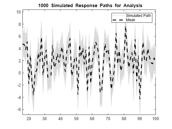
figure
h1 = plot(notBurnIn,var(U,0,2),'r','LineWidth',2);
hold on
h2 = plot([notBurnIn(1) notBurnIn(end)],...
    [theoVarFix theoVarFix],'k--','LineWidth',2);
title('{\bf Converged Unconditional Disturbance Variance}')
legend([h1,h2],'Simulation Variance','Theoretical Variance')
axis tight
hold off

Unconditional disturbance simulation variances fluctuate around the theoretical variance due to Monte Carlo sampling error. Be aware that the exclusion of the burn-in sample from analysis reduces the effective sample size.

Simulate an ARMA Error Model

This example shows how to simulate responses from a regression model with ARMA errors without specifying a presample.

Specify the regression model with ARMA(2,1) errors:

$$\begin{array}{l}{y}_t=2+X_t\left[\begin{array}{l}-2\\ 1.5\end{array}\right]+u_t\\ u_t=0.9u_{t-1}-0.1u_{t-2}+{\epsilon }_t+0.5{\epsilon }_{t-1},\end{array}$$

where $${\epsilon }_t$$ is distributed with 15 degrees of freedom and variance 1.

Beta = [-2; 1.5];
Intercept = 2;
a1 = 0.9;
a2 = -0.1;
b1 = 0.5;
Variance = 1;
Distribution = struct('Name','t','DoF',15);
Mdl = regARIMA('AR',{a1, a2},'MA',b1,...
    'Distribution',Distribution,'Intercept',Intercept,...
    'Beta',Beta,'Variance',Variance);

Generate two length T = 50 predictor series by random selection from the standard Gaussian distribution.

T = 50;
rng(6); % For reproducibility
X = randn(T,2);

The software treats the predictors as nonstochastic series.

Generate and plot one sample path of responses from Mdl.

rng(7);
ySim = simulate(Mdl,T,'X',X);

figure
plot(ySim)
title('{\bf Simulated Response Series}')

simulate requires:

• P = 2 presample unconditional disturbances to initialize the autoregressive component of the error series.

• Q = 1 presample innovations to initialize the moving average component of the error series.

Without them, as in this case, simulate sets the necessary presample errors to 0.

Alternatively, use filter to filter a random innovation series through Mdl.

rng(7);
e = randn(T,1);
yFilter = filter(Mdl,e,'X',X);

figure
plot(yFilter)
title('{\bf Simulated Response Series Using Filtered Innovations}')

The plots suggest that the simulated responses and the responses generated from the filtered innovations are equivalent.

Simulate 1000 response paths from Mdl. Assess transient effects by plotting the unconditional disturbance (U) variances across the simulated paths at each period.

numPaths = 1000;
[Y,~,U] = simulate(Mdl,T,'NumPaths',numPaths,'X',X);

figure
h1 = plot(Y,'Color',[.85,.85,.85]);
title('{\bf 1000 Simulated Response Paths}')
hold on
h2 = plot(1:T,Intercept+X*Beta,'k--','LineWidth',2);
legend([h1(1),h2],'Simulated Path','Mean')
hold off

figure
h1 = plot(var(U,0,2),'r','LineWidth',2);
hold on
theoVarFix = Variance*(a1*b1*(1+a2)+(1-a2)*(1+a1*b1+b1^2))/...
    ((1+a2)*((1-a2)^2-a1^2));
h2 = plot([1 T],[theoVarFix theoVarFix],'k--','LineWidth',2);
title('{\bf Unconditional Disturbance Variance}')
legend([h1,h2],'Simulation Variance','Theoretical Variance',...
    'Location','Best')
hold off

The simulated paths follow their theoretical mean, $$c+X\beta$$, which is not constant over time (and might look nonstationary).

The variance of the process is not constant, but levels off at the theoretical variance by the 10th period. The theoretical variance of the ARMA(2,1) error model is:

$$\frac{{\sigma }_{\epsilon }^2\left[a_1{b}_1\left(1+a_2\right)+\left(1-a_2\right)\left(1+a_1{b}_1+b_1^2\right)\right]}{{\left(1+a_2\right)}^2\left[{\left(1-a_2\right)}^2-a_1^2\right]}=\frac{\left[0.9(0.5)\left(1-0.1\right)+\left(1+0.1\right)\left(1+0.9(0.5)+{0.5}^2\right)\right]}{{\left(1-0.1\right)}^2\left[{\left(1+0.1\right)}^2-{0.9}^2\right]}=6.32.$$

You can reduce transient effects by partitioning the simulated data into a burn-in portion and a portion for analysis. Do not use the burn-in portion for analysis. Include enough periods in the burn-in portion to overcome the transient effects.

burnIn = 1:10;
notBurnIn = burnIn(end)+1:T;
Y = Y(notBurnIn,:);
X = X(notBurnIn,:);
U = U(notBurnIn,:);
figure
h1 = plot(notBurnIn,Y,'Color',[.85,.85,.85]);
hold on
h2 = plot(notBurnIn,Intercept+X*Beta,'k--','LineWidth',2);
title('{\bf 1000 Simulated Response Paths for Analysis}')
legend([h1(1),h2],'Simulated Path','Mean')
axis tight
hold off

figure
h1 = plot(notBurnIn,var(U,0,2),'r','LineWidth',2);
hold on
h2 = plot([notBurnIn(1) notBurnIn(end)],...
    [theoVarFix theoVarFix],'k--','LineWidth',2);
title('{\bf Converged Unconditional Disturbance Variance}')
legend([h1,h2],'Simulation Variance','Theoretical Variance')
axis tight
hold off

Unconditional disturbance simulation variances fluctuate around the theoretical variance due to Monte Carlo sampling error. Be aware that the exclusion of the burn-in sample from analysis reduces the effective sample size.