Incorporate Nonlinear View Constraints Using Sequential Entropy Pooling

R2026b

This example shows how to iterate the entropy pooling algorithm to incorporate nonlinear view constraints using functionality in Financial Toolbox™. When volatility views are imposed on a prior distribution, the algorithm uses the prior mean to build the second-moment constraint, which can cause the volatility view not to be satisfied if the posterior mean shifts. In this case, you can use a sequential approach to satisfy the volatility view by iterating until convergence.

Entropy Pooling

Entropy pooling [1] updates an empirical distribution to reflect user-specified views. Starting from a set of $$J$$ scenarios with prior probability weights $$q=\left(q_1,q_2,\dots ,q_J\right)$$, the entropy pooling algorithm finds posterior weights $$p=\left(p_1,p_2,\dots ,p_J\right)$$ that satisfy the user-specified view constraints while staying as close as possible to the prior, as measured by relative entropy (Kullback–Leibler divergence). Specifically, the algorithm finds posterior weights $$p$$ that minimize

$$\underset{j=1}{\sum ^J}{p}_j\ln \frac{p_j}{q_j}\text{,}\text{subject}\text{to}\text{the}\text{user}\text{-}\text{specified}\text{view}\text{constraints}\text{and}\underset{j=1}{\sum ^J}{p}_j=1\text{.}$$

$$Each user-specified view is modeled as a linear constraint on the posterior weights. For example, a mean view on variable $$i$$ takes the form of a first-moment constraint:

$$\underset{j=1}{\sum ^J}{p}_j{x}_{j,i}={\mu }_{i\text{,}\text{target}}\text{,}\text{where}{\mu }_{i\text{,}\text{target}}\text{is}\text{the}\text{target}\text{mean.}$$

The resulting posterior alters the prior as little as possible while satisfying every view. To create and solve this type of problem you use the entropyViews object.

Limitations When Volatility Views Are Imposed

To see the limitations of the entropy pooling algorithm, create a simple scenario set and impose both a mean view and a volatility view. Start by generating normally distributed scenarios for a single variable with a nonzero mean.

rng("default")
nScenarios = 100000;
returns = randn(nScenarios,1)+0.5; % Prior: mean ~0.5, std ~1

Create an entropyViews object with uniform (default) prior weights.

ev = entropyViews(returns,VariableNames="Returns");

Impose a mean view of 1 and a volatility (standard deviation) view of 1.2. Use the setMeanViews and setVolatilityViews functions to add these views to the object.

targetMean = 1; % Prior mean is ~0.5.
targetVol = 1.2; % Prior volatility is ~1.
ev = setMeanViews(ev,"Returns","=",targetMean);
ev = setVolatilityViews(ev,"Returns","=",targetVol);

Solve for the posterior weights using the posteriorProbabilities function, and compute the posterior mean and standard deviation.

p = posteriorProbabilities(ev);
posteriorMean = mean(returns,1,Weights=p)

posteriorMean = 
1.0000

posteriorStd = std(returns,p)

posteriorStd = 
0.8302

The posterior mean matches the target mean of 1 exactly, but the posterior standard deviation does not match the target volatility of 1.2 exactly. Rather, the posterior standard deviation only approximates the target volatility.

Why Volatility Views Are Approximate

Given the identity $$E\left[X_i^2\right]=E{\left[X_i\right]}^2+Var\left[X_i\right]\text{,}$$ a volatility view on variable $$i$$ takes the form of a second-moment constraint:

$$\underset{j=1}{\sum ^J}{p}_j{x}_{j,i}^2={\mu }_{i\text{,}\text{posterior}}^2+{\sigma }_{i\text{,}\text{target}}^2\text{,}\text{where}{\mu }_{i\text{,}\text{posterior}}\text{and}{\sigma }_{i\text{,}\text{target}}\text{are}\text{the}\text{posterior}\text{mean}\text{and}\text{target}\text{standard}\text{deviation,}\text{respectively.}$$

However, the constraint set by the setVolatilityViews function is an approximation, taking the form

$$\underset{j=1}{\sum ^J}{p}_j{x}_{j,i}^2={\mu }_{i\text{,}\text{prior}}^2+{\sigma }_{i\text{,}\text{target}}^2\text{,}\text{where}{\mu }_{i\text{,}\text{prior}}\text{is}\text{the}\text{prior}\text{mean.}$$

This approximation occurs because the entropy pooling algorithm requires the constraint equations to be linear in $$p$$, and $${\mu }_{i\text{,}\text{posterior}}^2$$ is a nonlinear function of $$p$$. Replacing $${\mu }_{i\text{,}\text{posterior}}$$ with $${\mu }_{i\text{,}\text{prior}}$$ (which is a constant) in the equation, following [1], makes the equation linear in $$p$$. Therefore, when the algorithm shifts the posterior mean away from the prior mean, the second-moment target is no longer consistent with the requested volatility, and the achieved standard deviation is off.

To verify this statement, check that the second-moment constraint was satisfied. The constraint targets $${\mu }_{i\text{,}\text{prior}}^2+{\sigma }_{i\text{,}\text{target}}^2\text{,}$$ so compare the posterior second moment against that value directly.

priorMean = mean(returns);
posteriorSecondMoment = mean(returns.^2,1,Weights=p)

posteriorSecondMoment = 
1.6892

constraintTarget = priorMean^2+targetVol^2

constraintTarget = 
1.6892

The two values match, confirming that the solver satisfied the second-moment constraint exactly. The difference between the posterior standard deviation and the target volatility arises because the volatility constraint is built using the prior mean instead of the posterior mean.

The strategy to correct this difference depends on whether a mean view is present.

• When a mean view is present, the posterior mean is known in advance. In this case, a single additional iteration suffices to correct the difference.

• When a mean view is not present, the posterior mean is not known in advance and can shift as a side effect of reweighting. In this case, iteration until convergence corrects the difference.

Sequential Entropy Pooling When Mean View Is Present

When a mean view is present, the posterior mean is known in advance because it is fixed by the view. In this case, you can correct the second-moment target in a single additional solve [2] by completing these steps:

1. Solve with only the mean view to obtain posterior values with the correct mean.

2. Use the posteriors as the new priors by passing the posterior weights using the PriorProbabilities name-value argument, and impose the volatility view in addition to the mean view. Because the prior mean now equals the posterior mean, the second-moment target is correct.

First, solve with just the mean view.

evMean = entropyViews(returns,VariableNames="Returns");
evMean = setMeanViews(evMean,"Returns","=",targetMean);
pMean = posteriorProbabilities(evMean);

Now perform the sequential solve. Use these posterior weights as the priors, and impose both the mean and volatility views.

pMean = pMean/sum(pMean);
evSeq = entropyViews(returns,VariableNames="Returns",PriorProbabilities=pMean);
evSeq = setMeanViews(evSeq,"Returns","=",targetMean);
evSeq = setVolatilityViews(evSeq,"Returns","=",targetVol);
pSeq = posteriorProbabilities(evSeq);

Check the results.

posteriorMeanSeq = mean(returns,1,Weights=pSeq)

posteriorMeanSeq = 
1.0000

posteriorStdSeq = std(returns,pSeq)

posteriorStdSeq = 
1.2000

Both the mean and volatility now match their targets.

Visualize the changes to the posterior distribution by using the local function plotPosteriorComparison, defined at the end of this example.

plotPosteriorComparison(returns,p,pSeq,"Effect of Sequential Entropy Pooling on Posterior Distribution")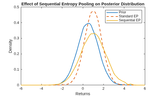

Sequential Entropy Pooling When Mean View Is Not Present

When a mean view is not present, the posterior mean is not fixed and, therefore, it can shift as a side effect of reweighting. Each correction to the second-moment target changes the posterior mean, which in turn changes the target again. The solution is to iterate until both the achieved mean and volatility stabilize [2].

Start by solving with just the volatility view, and then iterate on the posteriors until convergence.

pIter = ones(nScenarios,1); % Start with uniform priors.
maxIter = 50;
tol = 1e-6;
iterResults = table(Size=[maxIter 4],VariableTypes=repmat("double",1,4),VariableNames=["Iteration" "Mean" "Std" "Error"]);

for k = 1:maxIter
    % Set up and solve the latest iteration of the entropy pooling problem.
    pIter = pIter/sum(pIter); % Normalize the probabilities.
    evIter = entropyViews(returns,VariableNames="Returns",PriorProbabilities=pIter);
    evIter = setVolatilityViews(evIter,"Returns","=",targetVol);
    pIter = posteriorProbabilities(evIter);

    % Calculate the updated mean and volatility, and check for convergence.
    iterResults.Iteration(k) = k;
    iterResults.Mean(k) = mean(returns,1,Weights=pIter);
    iterResults.Std(k) = std(returns,pIter);
    iterResults.Error(k) = abs(iterResults.Std(k)-targetVol);

    if iterResults.Error(k) < tol
        break
    end
end

Summarize the results in a table.

iterResults = iterResults(1:k,:);
disp(iterResults)

    Iteration     Mean       Std        Error   
    _________    _______    ______    __________

        1        0.64257    1.1297      0.070262
        2        0.69224     1.172      0.027952
        3        0.71199    1.1884      0.011608
        4        0.72018    1.1951     0.0049002
        5        0.72364    1.1979     0.0020825
        6        0.72511    1.1991    0.00088754
        7        0.72574    1.1996     0.0003787
        8          0.726    1.1998    0.00016164
        9        0.72612    1.1999    6.9018e-05
       10        0.72617       1.2    2.9434e-05
       11        0.72619       1.2    1.2531e-05
       12         0.7262       1.2    5.3214e-06
       13         0.7262       1.2    2.2426e-06
       14         0.7262       1.2     9.182e-07

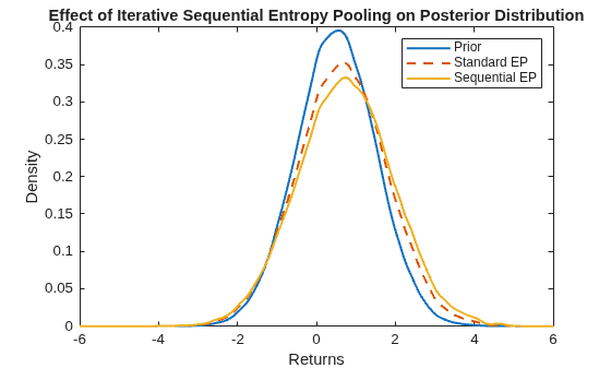
The posterior standard deviation now matches the target. The posterior mean shifted from the prior mean due to the reweighting, because no mean view was present.

To visualize the improvement, solve the standard (nonsequential) problem for comparison, and plot both posteriors.

evVolOnly = entropyViews(returns,VariableNames="Returns");
evVolOnly = setVolatilityViews(evVolOnly,"Returns","=",targetVol);
pVolOnly = posteriorProbabilities(evVolOnly);
plotPosteriorComparison(returns,pVolOnly,pIter,"Effect of Iterative Sequential Entropy Pooling on Posterior Distribution")

References

1. Meucci, A. "Fully Flexible Views: Theory and Practice." Risk. Vol. 21, Number 10, 2008, pp. 97–102. Available at SSRN: https://ssrn.com/abstract=1213325.

2. Vorobets, A. "Sequential Entropy Pooling Heuristics." October 2021. Available at SSRN: https://ssrn.com/abstract=3936392.

Local Functions

function plotPosteriorComparison(returns,pStandard,pSequential,titleStr)
% Interpolation points for plot
xi = linspace(-6,6,500)';

% Density function estimates
fPrior = ksdensity(returns,xi);
fStandard = ksdensity(returns,xi,Weights=pStandard);
fSequential = ksdensity(returns,xi,Weights=pSequential);

% Plot density functions
figure
plot(xi,fPrior,xi,fStandard,"--",xi,fSequential,LineWidth=1.5)
legend("Prior","Standard EP","Sequential EP")
xlabel("Returns")
ylabel("Density")
title(titleStr)
end