Track Space Debris Using a Keplerian Motion Model
R2026bThis example shows how to simulate space debris with trackingScenario and how to configure a fusionRadarSensor in monostatic mode to generate synthetic detections of space debris. The example also shows how to configure a task-oriented multi-object tracker to track the simulated debris.
Space Debris Scenario
There are more than 30,000 large debris objects (with diameter larger than 10 cm) and more than 1 million smaller debris objects in Low Earth Orbit (LEO) [1]. This debris poses a danger to human activities in space, damages operational satellites, and forces time-sensitive and costly avoidance maneuvers. As space activity increases, reducing and monitoring space debris becomes crucial.
You can use Sensor Fusion and Tracking Toolbox™ and Aerospace Toolbox to model the debris trajectories, generate synthetic radar detections of the debris, and track position and velocity estimates of all debris.
Create Tracking Scenario
First, create a tracking scenario and set the random seed for repeatable results. Set the IsEarthCentered property to true to model trajectories with respect to Earth.
seed = 2020;
rng(seed);
tTotal = 1800; % seconds
dt = 4; % seconds
updateRate = 1/dt; % Hz
scene = trackingScenario(IsEarthCentered=true, InitialAdvance="UpdateInterval",...
    StopTime=tTotal, UpdateRate=updateRate);
Define Space Debris
First, generate the initial states for 100 space debris objects by varying their orbital elements: semi-major axis, eccentricity, inclination, right ascension of ascending node, argument of periapsis, and true anomaly. These orbits are nearly circular low-Earth orbits with an orbital period of roughly 100 minutes.
numDebris = 100;

a = 7e6 + 1e5*randn(numDebris,1); % semi-major axis
ecc = abs(0.015 + 0.005*randn(numDebris,1)); % eccentricity
inc = 80 + 10*rand(numDebris,1); % inclination
raan = 360*rand(numDebris,1); % right ascension of ascending node
w = 360*rand(numDebris,1); % argument of periapsis
nu = 360*rand(numDebris,1); % true anomaly
Propagate the orbits of these debris by using the propagateOrbit function. Assume the initial time epoch is at 13-May-2026 08:36:36. As demonstrated in the next section, this example uses four ground-based radar stations to detect the debris. To enable this, transform the positions and velocities from the Earth-Centered Inertial (ECI) frame to geodetic coordinates (latitude, longitude, and altitude) and the corresponding velocities in the North-East-Down (NED) frame.
utc0 = datetime(2026,5,13,8,36,36);
utcs = utc0 + seconds(0:dt:tTotal);
[lla,velocitiesNED] = propagateOrbit(utcs,a,ecc,inc,raan,w,nu,OutputCoordinateFrame="geographic",PropModel="two-body-keplerian");
Now, define the debris as platforms in the tracking scenario. Assign a trajectory to each platform using geoTrajectory objects.
timeOfArrivals = seconds(utcs-utcs(1)); % Obtain time in seconds
for ii=1:numDebris
    debris(ii) = platform(scene); %#ok<SAGROW>
    debris(ii).Trajectory = geoTrajectory(lla(:,:,ii)',timeOfArrivals,Velocities=velocitiesNED(:,:,ii)'); %#ok<SAGROW>
end
Model Space Surveillance Radars
Define four antipodal stations with fan-shaped radar beams looking into space. The fans cut through the orbits of debris to maximize the number of debris detections. A pair of stations are located in the Pacific Ocean and in the Atlantic Ocean, whereas a second pair of surveillance stations is located near the poles. Having four dispersed radars allows for the re-detection of space debris to correct their position estimates and to acquire acquiring new debris detections.
% Specify four station positions in latitude, longitude, and altitude.
stationsLLA = [10 180 0;
                0 -20 0;
               65 -20 0;
              -90   0 0];
% Create a space surveillance station in the Pacific ocean.
station1 = platform(scene,Position=stationsLLA(1,:));
% Create a second surveillance station in the Atlantic ocean.
station2 = platform(scene,Position=stationsLLA(2,:));
% Near the North Pole, create a third surveillance station in Iceland.
station3 = platform(scene,Position=stationsLLA(3,:));
% Create a fourth surveillance station near the South Pole.
station4 = platform(scene,Position=stationsLLA(4,:));
Each station has a radar, modeled using a fusionRadarSensor object. To detect debris objects in the LEO range, the radar has the following requirements:
Detecting a 10 dBsm object up to 2000 km away
Resolving objects horizontally and vertically with a precision of 100 m at 2000 km range
Having a fan-shaped field of view of 120 degrees in azimuth and 30 degrees in elevation
Looking up into space based on its geo-location
Reporting detections in azimuth, elevation, and range
% Create fan-shaped monostatic radars to monitor space debris objects
radar1 = fusionRadarSensor(1,...
    UpdateRate=updateRate,...
    ScanMode="No scanning",...
    MountingAngles=[0 90 0],... % Look up
    FieldOfView=[120;30],... % degrees
    ReferenceRange=2e6,... % m
    RangeLimits=[0 2e6],...
    ReferenceRCS=10,... % dBsm
    HasFalseAlarms=false,...
    HasElevation=true,...
    AzimuthResolution=0.01,... % degrees
    ElevationResolution=0.01,... % degrees
    RangeResolution=100,... % m
    HasINS=true,...
    DetectionCoordinates="Sensor Spherical");
station1.Sensors = radar1;

radar2 = clone(radar1);
radar2.SensorIndex = 2;
station2.Sensors = radar2;

radar3 = clone(radar1);
radar3.SensorIndex = 3;
station3.Sensors = radar3;

radar4 = clone(radar1);
radar4.SensorIndex = 4;
station4.Sensors = radar4;
Visualize the Ground Truth with trackingGlobeViewer
You can use trackingGlobeViewer to visualize all the elements defined in the tracking scenario: individual debris objects and their trajectories, radar fans, radar detections, and tracks.
f = uifigure;
viewer = trackingGlobeViewer(f,Basemap="satellite",ShowDroppedTracks=false,NumCovarianceSigma=3);
% Add info box on top of the globe viewer
infotext = simulationInfoText(0,0,0);
infobox = uilabel(f,Text=infotext,FontColor=[1 1 1],FontSize=11,...
    Position=[10 20 300 70],Visible="on");

% Show radar beams on the globe
coverages = coverageConfig(scene);
plotCoverage(viewer, coverages, "ECEF");
scene.restart();
% Simulate the debris motion
while advance(scene)
    infobox.Text = simulationInfoText(scene.SimulationTime, 0, numDebris);
    plotPlatform(viewer, debris, "ECEF","TrajectoryMode","History");
end
% Take a snapshot of the scenario
snapshot(viewer);
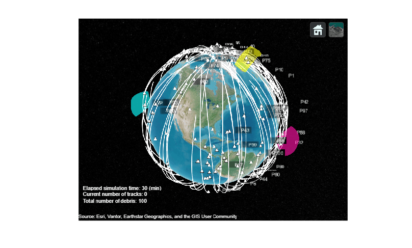
On the virtual globe, space debris is visualized as white dots. Most of these generated objects follow orbits with high inclination angles, close to 80 degrees. The trajectories are plotted in Earth-Centered, Earth-Fixed (ECEF) coordinates, and so the entire trajectory drifts westward due to Earth’s rotation. Over several orbital periods, all debris objects will eventually pass through the surveillance beams of the radars.
Define Tracker
To track these debris, you can use a task-oriented multi-object tracker which integrates data from multiple sensors and creates a unified representation of target states. The tracker processes incoming sensor data by:
Evaluating existing tracks
Associating new data with them
Updating tracks using filtering techniques such as Kalman filtering
Adjusting track existence probabilities based on sensor field-of-view
Initiating new tracks for unassigned detections

Specify Target Type
In this step, you specify the type and the characteristics of the objects you intend to track, which informs the tracker about choosing appropriate models and parameters to define the target. You use the trackerTargetSpec function to create a target spec that models Keplerian motion.
debrisSpec = trackerTargetSpec("space","earth-centered","keplerian");
disp(debrisSpec)
  EarthCenteredKeplerian with properties:

                   MinAltitude: 1.2e+05    m
                   MaxAltitude: 2e+06      m
                      MaxSpeed: 8000       m/s
    MaxDisturbanceAcceleration: 0.02       m/s²
The display above shows the list of properties of the Keplerian target specification, which can be modified for your application. The specification models target states as in the ECI frame. The MinAltitude and MaxAltitude properties specify the region of interest for tracking. Targets that fall outside this altitude range are assigned a low survival probability and are likely to be quickly removed by the tracker that uses this target specification. The MaxSpeed property sets the upper limit for the magnitude of a target’s initial velocity. The MaxDisturbanceAcceleration property defines the extent of motion uncertainty, accounting for unmodeled perturbations such as higher-order gravitational effects, atmospheric drag, and solar radiation pressure.
Specify Sensor Type
After specifying the objects to track, you specify the sensors you use for tracking. First, use the trackerSensorSpec function to create the monostatic radar specification for the first radar.
radarSpec1 = trackerSensorSpec("space","ground-based","radar");
disp(radarSpec1)
  SpaceGroundBasedRadar with properties:

           MaxNumLooksPerUpdate: 30
    MaxNumMeasurementsPerUpdate: 10

              ReferenceFrame: 'NED'
       GroundStationPosition: [0 0 0]         [deg deg m]
    GroundStationOrientation: [3⨯3 double]
            MountingLocation: [0 0 0]         m
              MountingAngles: [0 0 0]         deg

       HasElevation: 1
       HasRangeRate: 1
        FieldOfView: [60 20]           deg
        RangeLimits: [1e+05 2e+06]     m
    RangeRateLimits: [-10000 10000]    m/s

      AzimuthResolution: 1      deg
        RangeResolution: 100    m
    ElevationResolution: 5      deg
    RangeRateResolution: 10     m/s

    DetectionProbability: 0.9
          FalseAlarmRate: 1e-06

    Terrain: 'none'
Then, specify the characteristics of the sensor spec based on the sensors you simulated in the last section.
radarSpec1.GroundStationPosition = stationsLLA(1,:);
radarSpec1.MountingAngles = [0 90 0];
radarSpec1.HasRangeRate = false;
radarSpec1.FieldOfView = [120;30];
radarSpec1.RangeLimits = [0 2e6];
radarSpec1.AzimuthResolution = 0.01;
radarSpec1.ElevationResolution = 0.01;
radarSpec1.RangeResolution = 100;
radarSpec1.BirthRate = 1e-10;
radarSpec1.FalseAlarmRate = 1e-10;
All the other sensors only differ from the first sensor by ground station position. So, you create copies of the first sensor spec and modify their ground station positions.
radarSpec2 = radarSpec1;
radarSpec2.GroundStationPosition = stationsLLA(2,:);

radarSpec3 = radarSpec1;
radarSpec3.GroundStationPosition = stationsLLA(3,:);

radarSpec4 = radarSpec1;
radarSpec4.GroundStationPosition = stationsLLA(4,:);
Configure Tracker
In this step, you create a tracker based on the created target spec and sensor specs. Also, you choose to use the joint integrated probabilistic data association (JIPDA) algorithm.
tracker = multiSensorTargetTracker(debrisSpec,{radarSpec1,radarSpec2,radarSpec3,radarSpec4},"jipda");Using the target specifications, the tracker configures the right motion and survival models. Also, the sensor specifications provide the right observability, measurement, clutter, birth, and state initialization models to the tracker.
disp(tracker)
  fusion.tracker.JIPDATracker with properties:

                TargetSpecifications: {[1×1 EarthCenteredKeplerian]}
                SensorSpecifications: {[1×1 SpaceGroundBasedRadar]  [1×1 SpaceGroundBasedRadar]  [1×1 SpaceGroundBasedRadar]  [1×1 SpaceGroundBasedRadar]}
              MaxMahalanobisDistance: 5
    ConfirmationExistenceProbability: 0.9000
        DeletionExistenceProbability: 0.1000
In addition to the target and sensor specifications, the tracker exposes tuning parameters to help control data association, track confirmation, and track deletion. The MaxMahalanobisDistance property controls the size of the association gate. Generally, this distance should be small to limit the association gate, but if you observe that the tracker fails to associate a measurement to the track, you can increase this value slightly. The ConfirmationExistenceProbability property defines the probability threshold to confirm a track. The DeletionExistenceProbability property defines the probability threshold to remove a track.
Sensor Data Format
The sensor specifications determine the format of sensor data that the tracker expects. You can display the data format by using the dataFormat() object function of the sensor specification.
format = dataFormat(radarSpec1)
format = struct with fields:
             LookTime: [01-Jan-1970    01-Jan-1970    01-Jan-1970    01-Jan-1970    01-Jan-1970    01-Jan-1970    01-Jan-1970    01-Jan-1970    01-Jan-1970    01-Jan-1970    01-Jan-1970    01-Jan-1970    01-Jan-1970    …    ] (1×30 datetime)
          LookAzimuth: [0 0 0 0 0 0 0 0 0 0 0 0 0 0 0 0 0 0 0 0 0 0 0 0 0 0 0 0 0 0]
        LookElevation: [0 0 0 0 0 0 0 0 0 0 0 0 0 0 0 0 0 0 0 0 0 0 0 0 0 0 0 0 0 0]
        DetectionTime: [01-Jan-1970    01-Jan-1970    01-Jan-1970    01-Jan-1970    01-Jan-1970    01-Jan-1970    01-Jan-1970    01-Jan-1970    01-Jan-1970    01-Jan-1970]
              Azimuth: [0 0 0 0 0 0 0 0 0 0]
            Elevation: [0 0 0 0 0 0 0 0 0 0]
                Range: [0 0 0 0 0 0 0 0 0 0]
      AzimuthAccuracy: [0 0 0 0 0 0 0 0 0 0]
    ElevationAccuracy: [0 0 0 0 0 0 0 0 0 0]
        RangeAccuracy: [0 0 0 0 0 0 0 0 0 0]
The data format captures everything you need to provide for sensor scanning and measurements. It includes fields to specify the sensor's scanning information and measurement information. Each of these fields is populated with nominal values to match the MaxNumLooksPerUpdate and MaxNumMeasurementsPerUpdate values set in the sensor specification.
Next, you generate a recording of the scenario used in this example.
tsr = record(scene,IncludeSensors=true,RecordingFormat="Recording",InitialSeed=seed);Then, you organize the recorded sensor data by using the supporting function, helperOrganizeSensorData. The returned values, data1, data2, data3, and data4, follow the required data format.
[data1, data2, data3, data4] = helperOrganizeSensorData(tsr,format,utc0);
Run Tracker
Before running the tracker, you can tune these tracker properties.
release(tracker); tracker.DeletionExistenceProbability =0.1; tracker.ConfirmationExistenceProbability =
0.9; tracker.MaxMahalanobisDistance =
5;
Next, update the tracker using the sensor data and update the globe display.
reset(tsr);
clear(viewer);
snapshots = {};
plotCoverage(viewer,coverages,"ECEF");
for ii = 1:numel(data1)
    % Update tracker with sensor data
    confTracks = tracker(data1(ii),data2(ii),data3(ii),data4(ii));

    % Update Visualization
    % Read recording and plot debris poses
    [simulationTime,poses,~,detections] = read(tsr);
    plotPlatform(viewer, poses, "ECEF");
    % Plot sensor data
    plotSensorData(viewer,{data1(ii),data2(ii),data3(ii),data4(ii)},{radarSpec1,radarSpec2,radarSpec3,radarSpec4});
    % Plot confirmed tracks
    if ~isempty(confTracks)
        plotTrack(viewer,confTracks,debrisSpec,LabelStyle="Custom",CustomLabel="T" + string([confTracks.TrackID]));
    end
    % Update the info
    infobox.Text = simulationInfoText(simulationTime, numel(confTracks), numDebris);
    % Take and save snapshots at a few epochs
    snapshots = takeSnapshots(snapshots, viewer, simulationTime);
end
imshow(snapshots{1});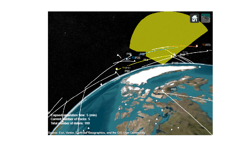
On the first snapshot, three debris passed through the surveillance region of the radar near Iceland. The tracker successfully created and maintained three tracks.
imshow(snapshots{2});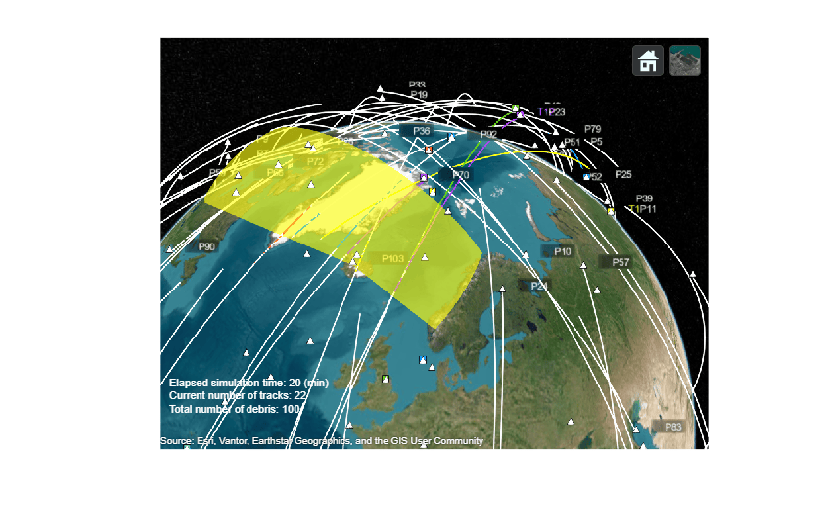
At approximately 20 minutes, the tracker tracks a total of 22 tracks.
imshow(snapshots{3});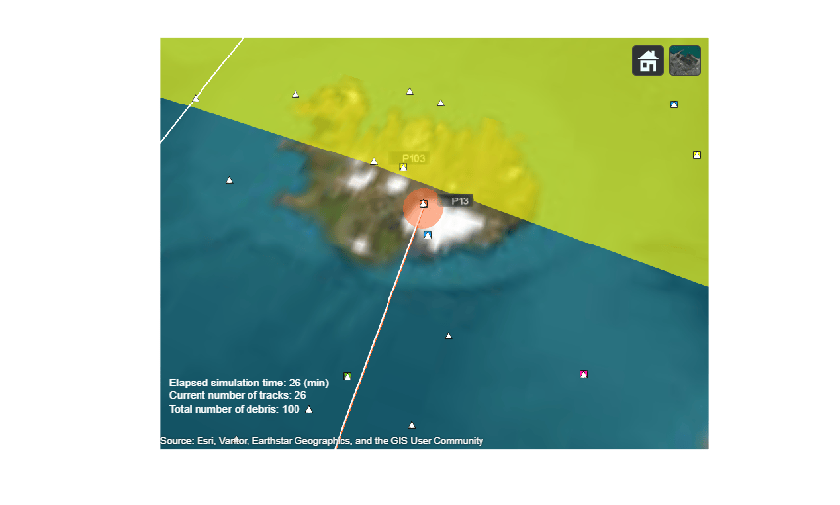
At approximately 26 minutes, track T10 was approaching the surveillance region of the Iceland radar. T10 was originally initialized in the coverage area of the Atlantic radar. After leaving the Atlantic radar’s coverage, the tracker continued to maintain and predict T10’s state. However, because T10 was outside the range of all sensors during this prediction period, its covariance ellipse expanded, indicating increased motion uncertainty.
imshow(snapshots{4});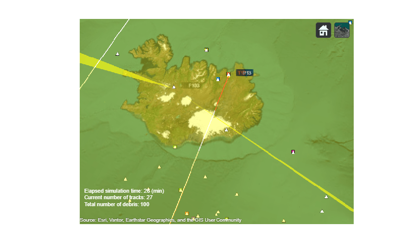
After 24 seconds, track T10 entered the surveillance region of the Iceland radar. The tracker successfully associated T10 with a new detection, resulting in a reduction of its motion uncertainty as expected.
imshow(snapshots{5});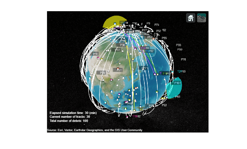
At the end of the simulation, the tracker maintains a total of 30 confirmed tracks out of 100 debris with the sparse radar station configuration. If you increase the simulation time, the radars cover more debris. Explore different radar station locations and configurations to increase the number of tracked objects.
The exported tracks include the actual track times in POSIX format, which can be easily converted to standard datetime values.
datetimeFinal = datetime(confTracks(1).UpdateTime,ConvertFrom="posixtime")datetimeFinal = datetime
13-May-2026 09:06:36
Supporting Functions
helperOrganizeSensorData Organize sensor data from the scenario to format required by sensor spec
function varargout = helperOrganizeSensorData(tsr, format, initialUTC)
% Extract recorded data from the tracking sensor report
data = tsr.RecordedData;

% Get field names from the format structure
fields = fieldnames(format);

% Initialize each field in the format structure with an empty array
for i = 1:length(fields)
    className = class(format.(fields{i}));
    format.(fields{i}) = feval([className,'.empty'],1,0);
end

% Determine the number of simulation steps and sensors
numSteps = numel(data);
numSensors = numel(data(1).SensorConfigurations);

% Initialize output cell array for each sensor
sensorData = cell(1, numSensors);

% Create a template structure for each sensor's data across all steps
for ii = 1:numSensors
    sensorData{ii} = repmat(format, numSteps, 1);
end

% Process data for each simulation step
for jj = 1:numSteps
    % Extract data for the current simulation step
    stepData = data(jj);
    simulationTime = stepData.SimulationTime;

    % Process coverage configuration data for each sensor
    for kk = 1:numel(stepData.CoverageConfig)
        configData = stepData.CoverageConfig(kk);
        index = configData.Index;

        % Assign look time and angles to the corresponding sensor's data
        sensorData{index}(jj).LookTime = initialUTC + seconds(simulationTime);
        sensorData{index}(jj).LookAzimuth = configData.LookAngle(1);
        sensorData{index}(jj).LookElevation = configData.LookAngle(2);

    end

    % Process detection data for the current step
    numDetections = numel(stepData.Detections);
    for kk = 1:numDetections
        detection = stepData.Detections{kk};
        index = detection.SensorIndex;

        % Append detection measurements and accuracies to the sensor's data
        sensorData{index}(jj).DetectionTime = [sensorData{index}(jj).DetectionTime ...
            initialUTC + seconds(detection.Time)];
        sensorData{index}(jj).Azimuth = [sensorData{index}(jj).Azimuth detection.Measurement(1)];
        sensorData{index}(jj).Elevation = [sensorData{index}(jj).Elevation detection.Measurement(2)];
        sensorData{index}(jj).Range = [sensorData{index}(jj).Range detection.Measurement(3)];

        factor = 1;
        azimuthAccuray = sqrt(detection.MeasurementNoise(1,1))*factor;
        elevationAccuracy = sqrt(detection.MeasurementNoise(2,2))*factor;
        rangeAccuracy = sqrt(detection.MeasurementNoise(3,3))*factor;

        sensorData{index}(jj).AzimuthAccuracy = [sensorData{index}(jj).AzimuthAccuracy azimuthAccuray];
        sensorData{index}(jj).ElevationAccuracy = [sensorData{index}(jj).ElevationAccuracy elevationAccuracy];
        sensorData{index}(jj).RangeAccuracy = [sensorData{index}(jj).RangeAccuracy rangeAccuracy];
    end
end
varargout = sensorData;
end
simulationInfoText Display the simulation time, the number of debris, and the current number of tracks in the scenario.
function text = simulationInfoText(time,numTracks, numDebris)
text = vertcat(string(['Elapsed simulation time: ' num2str(round(time/60)) ' (min)']),...
    string(['Current number of tracks: ' num2str(numTracks)]),...
    string(['Total number of debris: ' num2str(numDebris)]));
drawnow limitrate
end
takeSnapshots Move camera and take snapshots at a few time epochs
function snapshots = takeSnapshots(snapshots, viewer, simulationTime)
% Move camera during simulation and take snapshots
switch simulationTime
    case 272 % Good to keep
        campos(viewer,[60 -120 2.6e6]);
        camorient(viewer, [20 -45 20]);
        drawnow
        snap = snapshot(viewer);
        snapshots = [snapshots {snap}];
    case 1200
        campos(viewer,[54 2.3 6.09e6]);
        camorient(viewer, [0 -73 348]);
        drawnow
        snap = snapshot(viewer);
        snapshots = [snapshots {snap}];
    case 1544
        campos(viewer,[61.9142 -15.26258 7.614006e5]);
        camorient(viewer,[342.97078 -71.944895 0]);
        drawnow
        snap = snapshot(viewer);
        snapshots = [snapshots {snap}];
    case 1568
        campos(viewer,[63.380 -15.3023 7.614006e5]);
        camorient(viewer,[340.2416 -79.6413 0]);
        drawnow
        snap = snapshot(viewer);
        snapshots = [snapshots {snap}];
    case 1800
        campos(viewer,[0000044.75562659	125.72492074	1.5699123*1e7]);
        camorient(viewer,[360.0000  -89.9854833  0]);
        drawnow
        snap = snapshot(viewer);
        snapshots = [snapshots {snap}];
end
end
References
[1] https://www.esa.int/Space_Safety/Space_Debris/Space_debris_by_the_numbers

