Tune Fuzzy PID Controller to Meet Step-Response Requirements

R2026b

Since R2026b

This example uses:

This example shows how to programmatically optimize fuzzy PID controller parameters to meet step-response requirements using Simulink® Design Optimization™ software. This example is adapted from Design Optimization to Meet Step Response Requirements (Code) (Simulink Design Optimization).

Model Structure

This example uses the fpid_watertank_stepinput model, which includes a fuzzy PID controller block and a nonlinear water-tank system plant in a single-loop feedback configuration.

Load the model.

model = "fpid_watertank_stepinput";
load_system(model)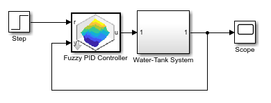

For more information on the water-tank system, see here.

The following figure shows the structure of the fuzzy PID controller, which is implemented using a Fuzzy PID Controller block.

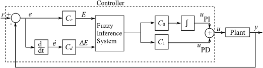
The continuous-time fuzzy PID controller includes these components:

Fuzzy inference system (FIS) a default linear control surface
Integrator block
Derivative block
Controller gains $C_{0}$ , $C_{1}$ , $C_{e}$ , and $C_{d}$

For this example, you keep the default FIS structure and tune the controller gains using Simulink Design Optimization methods.

To reduce the optimization time, the Fuzzy PID Controller block is configured to simulate as a lookup table. When you select the Implement FIS as lookup table block parameter, the FIS in the controller uses a lookup table for simulation, which is faster than performing the entire inference process during simulation.

Specify Step-Response Requirements

The height of water in the tank must meet the following step-response requirements:

Rise time less than 2.5 seconds
Settling time less than 20 seconds
Overshoot less than 5%

Specify the step-response requirements using an sdo.requirements.StepResponseEnvelope (Simulink Design Optimization) object.

stepResp = sdo.requirements.StepResponseEnvelope;
stepResp.RiseTime = 2.5;
stepResp.SettlingTime = 20;
stepResp.PercentOvershoot = 5;

Also, specify the initial and final values of the step response. These values correspond to the initial and final step values in the Step block of the model.

stepResp.FinalValue = 2;
stepResp.InitialValue = 1;

Configure Design Optimization Simulator

During optimization, the model is simulated using the current value of the model parameters and the logged signal is used to evaluate the design requirements.

For this model, log the water level, which is the output of the Water-Tank System block.

plantOutput = Simulink.SimulationData.SignalLoggingInfo;
plantOutput.BlockPath = model + "/Water-Tank System";
plantOutput.OutputPortIndex = 1;
plantOutput.LoggingInfo.NameMode = 1;
plantOutput.LoggingInfo.LoggingName = "PlantOutput";

Create an sdo.SimulationTest (Simulink Design Optimization) object to simulate the model and store the logged simulation data.

simulator = sdo.SimulationTest(model);
simulator.LoggingInfo.Signals = plantOutput;

Specify Design Variables

When you optimize the model response, the software modifies parameter (design variable) values to meet the design requirements.

Select the model parameters to optimize. Here, you optimize the gain parameters of the Fuzzy PID controller.

p = sdo.getParameterFromModel(model,["Ce","Cd","C0","C1"]);

p is an array of four param.Continuous objects.

To limit the gains to positive values, set the minimum value of each parameter to 0.

p(1).Minimum = 0;
p(2).Minimum = 0;
p(3).Minimum = 0;
p(4).Minimum = 0;

Optimize Model Response

Create a design function to evaluate the system performance for a set of parameter values.

evalDesign = @(p) fpidDesignFcn(p,simulator,stepResp);

evalDesign is an anonymous function that calls the cost function fpidDesignFcn. The cost function simulates the model and evaluates the design requirements. To view this function, type edit fpidDesignFcn at command line.

The fpidDesignFcn function returns a structure with inequality-constraint values in field Cleq. When all values in this field are less than zero, the simulation output satisfies the step-response requirements.

Compute the initial model response using the current values of the design variables.

initDesign = evalDesign(p);

Examine the nonlinear inequality constraints.

initDesign.Cleq

Some Cleq values are positive, which indicates that the response using the current parameter values violates the design requirements.

To confirm, you can view the plant output in the scope. The step response does not have the correct final value and has a long rise time.

open_system(model + "/Scope")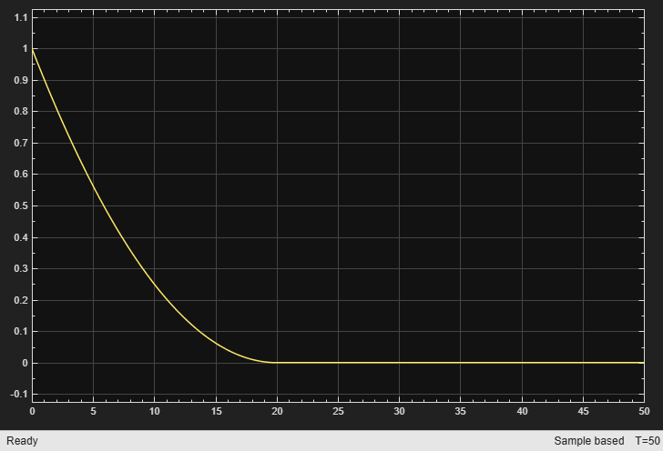

close_system(model + "/Scope")

Specify optimization options.

opt = sdo.OptimizeOptions;

For this example, use the default optimization method, fmincon (Optimization Toolbox) with the sequential quadratic programming (SQP) algorithm.

opt.MethodOptions.Algorithm = "sqp";

Optimize the response.

rng("default")
[pOpt,optInfo] = sdo.optimize(evalDesign,p,opt);

 Optimization started 2026-Jul-15, 10:04:28

                               max                     First-order 
 Iter F-count        f(x)   constraint    Step-size    optimality
    0      6            0        391.1
    1     14            0         34.9        0.259          416
    2     22            0       0.2371          1.4         20.7
    3     33            0       0.2944         1.39         2.12
    4     42            0       0.0688         1.11         3.62
    5     56            0      0.06349        0.365          2.5
    6     65            0     0.002208        0.592           38
    7     74            0    0.0001412        0.702       0.0765
    8     83            0            0        0.127      0.00823
    9     92            0            0     3.79e-12            0
Local minimum found that satisfies the constraints.

Optimization completed because the objective function is non-decreasing in 
feasible directions, to within the value of the optimality tolerance,
and constraints are satisfied to within the value of the constraint tolerance.

At each optimization iteration, the software simulates the model and the optimization solver modifies the design variables to meet the design requirements. For more information, see How the Optimization Algorithm Formulates Minimization Problems (Simulink Design Optimization).

The message Local minimum found that satisfies the constraints indicates that the optimization solver found a solution that meets the design requirements within specified tolerances. For more information about the outputs displayed during the optimization, see Iterative Display (Optimization Toolbox).

Examine the optimization termination information contained in the optInfo output argument. This information helps you verify that the response meets the step-response requirements.

For example, check the Cleq and exitflag fields.

Cleq shows the optimized nonlinear inequality constraints. Within the optimization tolerances, all values are less than or equal to zero, which indicates that the step-response requirements are satisfied.

optInfo.Cleq

exitflag identifies why the optimization terminated.

optInfo.exitflag

ans = 
1

The value is 1, which indicates that the solver found a solution that was less than the specified tolerances on the function value and constraint violations.

View the optimized parameter values.

pOpt

 
pOpt(1,1) =
 
       Name: 'Ce'
      Value: 2.4499
    Minimum: 0
    Maximum: Inf
       Free: 1
      Scale: 1
       Info: [1×1 struct]

 
pOpt(2,1) =
 
       Name: 'Cd'
      Value: 0.6229
    Minimum: 0
    Maximum: Inf
       Free: 1
      Scale: 1
       Info: [1×1 struct]

 
pOpt(3,1) =
 
       Name: 'C0'
      Value: 0.2192
    Minimum: 0
    Maximum: Inf
       Free: 1
      Scale: 1
       Info: [1×1 struct]

 
pOpt(4,1) =
 
       Name: 'C1'
      Value: 3.2805
    Minimum: 0
    Maximum: Inf
       Free: 1
      Scale: 1
       Info: [1×1 struct]

 
4x1 param.Continuous
 
lists of methods, superclasses

Simulate the model using the optimized values.

sdo.setValueInModel(model,pOpt);
sim(model);

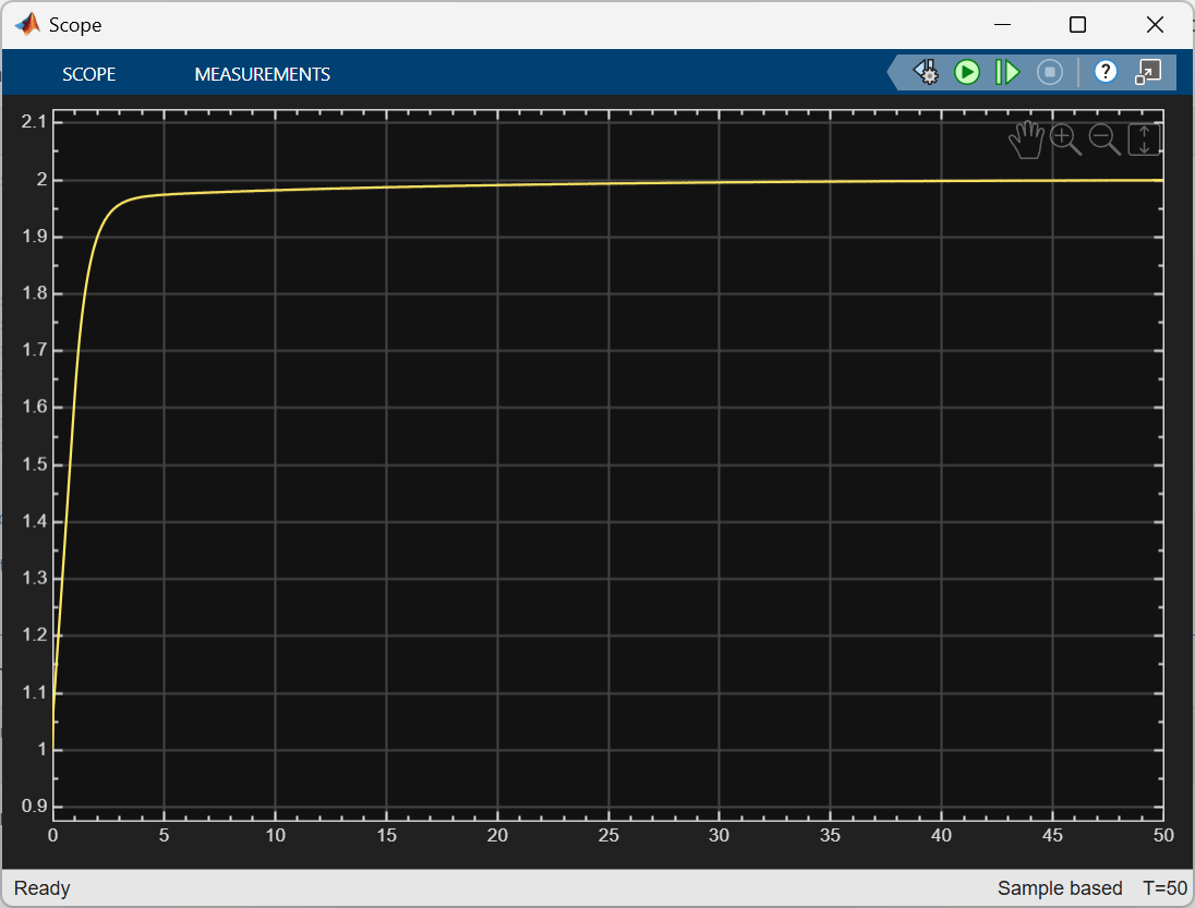
To verify that the model meets the step-response requirements, view the output signal. The plant output satisfies the rise-time, settling-time, and overshoot requirements. Also, it has the correct final value.

open_system(model + "/Scope")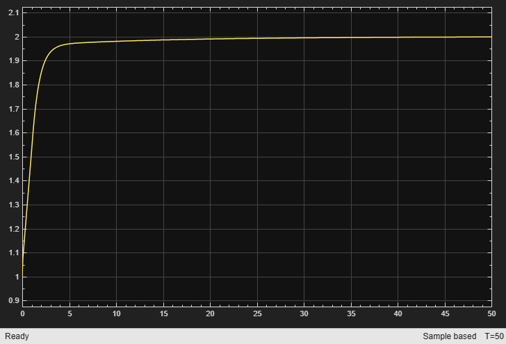

close_system(model + "/Scope")

Modify Optimization Configuration

The optimization results can change depending on the optimization algorithm used and the optimization settings.

Some changes can cause the optimization to not find a feasible solution. This is the case when you modify the initial controller gain values to be zero and use the fmincon method.

p(1,1).Value = 0;
[pOpt2,optInfo2] = sdo.optimize(evalDesign,p,opt);

 Optimization started 2026-Jul-15, 10:06:31

                               max                     First-order 
 Iter F-count        f(x)   constraint    Step-size    optimality
    0      5            0        391.1
    1      5            0        391.1            0            0
Converged to an infeasible point.

fmincon stopped because the size of the current step is less than
the value of the step size tolerance but constraints are not
satisfied to within the value of the constraint tolerance.

Changing the optimization method to patternsearch produces a different response that still satisfies the specified design requirements.

opt.Method = "patternsearch";
rng("default")
[pOpt3,optInfo3] = sdo.optimize(evalDesign,p,opt);

 Optimization started 2026-Jul-15, 10:06:43

 Phase one: Finding a feasible solution...


 Iter F-count        f(x)     MeshSize     Method
    0      1      391.054            1    
    1      3      12.6077            1   Successful Search
    2     54     0.154311            1   Successful Search
    3     94  -0.00471935            1   Successful Search
    4     95  -0.00483531            2   Successful Poll
    5     96  -0.00488053            4   Successful Poll
    6    100  -0.00488053            2   Refine Mesh
    7    104  -0.00488053            1   Refine Mesh
    8    106  -0.00489758            2   Successful Poll
    9    110  -0.00489758            1   Refine Mesh
   10    115  -0.00492748            2   Successful Poll
   11    116  -0.00496744            4   Successful Poll
   12    119  -0.00497139            8   Successful Poll
   13    123  -0.00497139            4   Refine Mesh
   14    127  -0.00497139            2   Refine Mesh
   15    131  -0.00497139            1   Refine Mesh
   16    137  -0.00497139          0.5   Refine Mesh
   17    140  -0.00497186            1   Successful Poll
   18    145  -0.00497186          0.5   Refine Mesh
   19    153  -0.00497186         0.25   Refine Mesh
   20    161  -0.00497186        0.125   Refine Mesh
   21    169  -0.00497186       0.0625   Refine Mesh
   22    177  -0.00497186       0.0312   Refine Mesh
   23    185  -0.00497186       0.0156   Refine Mesh
   24    193  -0.00497186      0.00781   Refine Mesh
   25    198  -0.00497198       0.0156   Successful Poll
   26    205  -0.00497198      0.00781   Refine Mesh
   27    213  -0.00497198      0.00391   Refine Mesh
   28    218  -0.00497205      0.00781   Successful Poll
   29    225  -0.00497205      0.00391   Refine Mesh
   30    233  -0.00497205      0.00195   Refine Mesh
   31    241  -0.00497205     0.000977   Refine Mesh
   32    246  -0.00497206      0.00195   Successful Poll
   33    253  -0.00497206     0.000977   Refine Mesh
   34    261  -0.00497206     0.000488   Refine Mesh
   35    266  -0.00497207     0.000977   Successful Poll
patternsearch stopped because the change in the objective function value was less than options.FunctionTolerance.

open_system(model + "/Scope")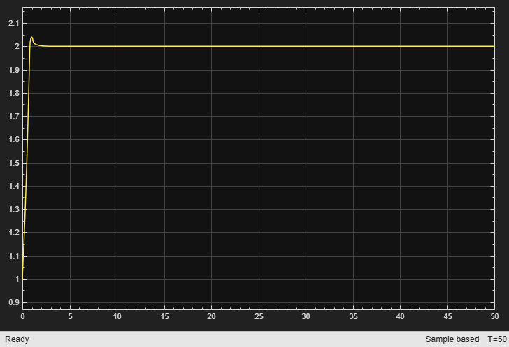

close_system(model + "/Scope")

Nonlinear Water-Tank Plant

The nonlinear plant is implemented in the Water-Tank System subsystem of the model. To view the system, open the subsystem.

open_system(model + "/Water-Tank System")

Water-tank System subsystem

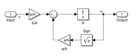
This model represents the following water tank system.

Water-tank system diagram

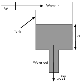
Here:

$Vol$ is the volume of water in the tank.
$A$ is the cross-sectional area of the tank.
$H$ is the height of water in the tank.
$V$ is the voltage applied to the pump.
$b$ is a constant related to the flow rate into the tank.
$a$ is a constant related to the flow rate out of the tank.

Water enters the tank at the top at a rate proportional to the valve opening. The valve opening is proportional to the voltage, $V$ , applied to the pump. The water leaves through an opening in the tank base at a rate that is proportional to the square root of the water height, $H$ . The presence of the square root in the water flow rate results in a nonlinear plant. Based on these flow rates, the rate of change of the tank volume is:

$\frac{d}{d t} Vol = A \frac{d}{d t} H = bV - a \sqrt{H}$ .

Tune Fuzzy PID Controller to Meet Step-Response Requirements

Model Structure

Specify Step-Response Requirements

Configure Design Optimization Simulator

Specify Design Variables

Optimize Model Response

Modify Optimization Configuration

Nonlinear Water-Tank Plant

See Also

Blocks

Functions

Topics