MultiStart Using lsqcurvefit or lsqnonlin

This example shows how to fit a function to data using lsqcurvefit together with MultiStart. The end of the example shows the same solution using lsqnonlin.

Many fitting problems have multiple local solutions. MultiStart can help find the global solution, meaning the best fit. This example first uses lsqcurvefit because of its convenient syntax.

The model is

$$y=a+b{x}_1\sin (c{x}_2+d),$$

where the input data is $$x=(x_1,x_2)$$, and the parameters $$a$$, $$b$$, $$c$$, and $$d$$ are the unknown model coefficients.

Step 1. Create the objective function.

Write an anonymous function that takes a data matrix xdata with N rows and two columns, and returns a response vector with N rows. The function also takes a coefficient matrix p, corresponding to the coefficient vector $$(a,b,c,d)$$.

fitfcn = @(p,xdata)p(1) + p(2)*xdata(:,1).*sin(p(3)*xdata(:,2)+p(4));

Step 2. Create the training data.

Create 200 data points and responses. Use the values $$a=-3,b=1/4,c=1/2,d=1$$. Include random noise in the response.

rng default % For reproducibility
N = 200; % Number of data points
preal = [-3,1/4,1/2,1]; % Real coefficients

xdata = 5*rand(N,2); % Data points
ydata = fitfcn(preal,xdata) + 0.1*randn(N,1); % Response data with noise

Step 3. Set bounds and initial point.

Set bounds for lsqcurvefit. There is no reason for $$d$$ to exceed $$\pi$$ in absolute value, because the sine function takes values in its full range over any interval of width $$2\pi$$. Assume that the coefficient $$c$$ must be smaller than 20 in absolute value, because allowing a high frequency can cause unstable responses or inaccurate convergence.

lb = [-Inf,-Inf,-20,-pi];
ub = [Inf,Inf,20,pi];

Set the initial point arbitrarily to (5,5,5,0).

p0 = 5*ones(1,4); % Arbitrary initial point
p0(4) = 0; % Ensure the initial point satisfies the bounds

Step 4. Find the best local fit.

Fit the parameters to the data, starting at p0.

[xfitted,errorfitted] = lsqcurvefit(fitfcn,p0,xdata,ydata,lb,ub)

Local minimum possible.

lsqcurvefit stopped because the final change in the sum of squares relative to 
its initial value is less than the value of the function tolerance.

<stopping criteria details>

xfitted = 1×4

   -2.6149   -0.0238    6.0191   -1.6998

errorfitted = 
28.2524

lsqcurvefit finds a local solution that is not particularly close to the model parameter values (–3,1/4,1/2,1).

Step 5. Set up the problem for MultiStart.

Create a problem structure so MultiStart can solve the same problem.

problem = createOptimProblem('lsqcurvefit','x0',p0,'objective',fitfcn,...
    'lb',lb,'ub',ub,'xdata',xdata,'ydata',ydata);

Step 6. Find a global solution.

Solve the fitting problem using MultiStart with 50 iterations. Plot the smallest error as the number of MultiStart iterations.

ms = MultiStart('PlotFcns',@gsplotbestf);
[xmulti,errormulti] = run(ms,problem,50)

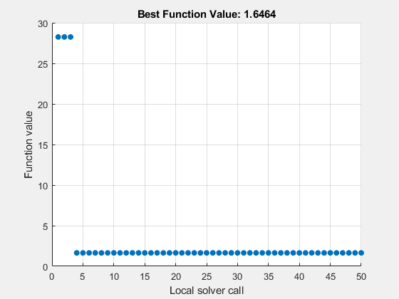
MultiStart completed the runs from all start points. 

All 50 local solver runs converged with a positive local solver exitflag.

xmulti = 1×4

   -2.9852   -0.2472   -0.4968   -1.0438

errormulti = 
1.6464

MultiStart finds a global solution near the parameter values (–3,–1/4,–1/2,–1). (This is equivalent to a solution near preal = (–3,1/4,1/2,1), because changing the sign of all the coefficients except the first gives the same numerical values of fitfcn.) The norm of the residual error decreases from about 28 to about 1.6, a decrease of more than a factor of 10.

Formulate Problem for lsqnonlin

For an alternative approach, use lsqnonlin as the fitting function. In this case, use the difference between predicted values and actual data values as the objective function.

fitfcn2 = @(p)fitfcn(p,xdata)-ydata;
[xlsqnonlin,errorlsqnonlin] = lsqnonlin(fitfcn2,p0,lb,ub)

Local minimum possible.

lsqnonlin stopped because the final change in the sum of squares relative to 
its initial value is less than the value of the function tolerance.

<stopping criteria details>

xlsqnonlin = 1×4

   -2.6149   -0.0238    6.0191   -1.6998

errorlsqnonlin = 
28.2524

Starting from the same initial point p0, lsqnonlin finds the same relatively poor solution as lsqcurvefit.

Run MultiStart using lsqnonlin as the local solver.

problem2 = createOptimProblem('lsqnonlin','x0',p0,'objective',fitfcn2,...
    'lb',lb,'ub',ub');
[xmultinonlin,errormultinonlin] = run(ms,problem2,50)

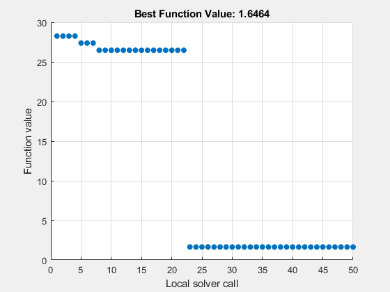
MultiStart completed the runs from all start points. 

All 50 local solver runs converged with a positive local solver exitflag.

xmultinonlin = 1×4

   -2.9852   -0.2472   -0.4968   -1.0438

errormultinonlin = 
1.6464

Again, MultiStart finds a much better solution than the local solver alone.