Upgrading Hydraulics (Isothermal) Models in Simscape Fluids
Learn how to use the hydraulicToIsothermalLiquid tool to upgrade Hydraulics (Isothermal) models. You
can convert multiple models at the same time.
The blocks in the Isothermal Liquid library account for density as a function of pressure, and pipe and actuator blocks account for compressibility by default. As a result, expect some differences between a model that uses Hydraulics (Isothermal) library blocks and a converted model when compressibility effects play a significant role due to the treatment of conservation equations in the volumetric-flow-rate-based and mass-flow-rate-based libraries.
These examples show how to run the conversion tool, respond to warning messages, and compare and check converted models with the Simulation Data Inspector.
Automatic Conversion
This example converts the Diesel Engine In-Line Injection System model and requires minimal manual adjustments.
Open the Diesel Engine In-Line Injection System model by entering
openExample('simscapefluids/DieselEngineInLineInjectionSystemHExample')at the MATLAB command line.Enable logging by clicking the signal line connected to the Scope block and clicking Log Signals on the Simulation tab.
Simulate the model.
On the Simulation tab, click Data Inspector.
To see one of the logged flow rates, expand Mux:1 and select Mux:1(1) to see the outlet flow rate in the
Injector Pump1subsystem.Convert the blocks in the model to the isothermal liquid library. At the command prompt, enter
hydraulicToIsothermalLiquid('DieselEngineInLineInjectionSystemH').The conversion report,
DieselEngineInLineInjectionSystemH_converted.html, opens when the model conversion completes. The report includes three types of warning messages:Predefined fluid has been reparameterized. Behavior change not expected at most temperatures.
This message indicates that the conversion process redefined the fluid for the Isothermal Liquid library in the Fuel Properties block in
DieselEngineInLineInjectionSystemH_converteddifferently, but no specific parameter requires user input.Critical Reynolds number set to 150. Behavior change not expected.
The conversion process converted the parameter that indicates flow regime to the Critical Reynolds number parameter. This parameter has a default value of 150. You do not need to adjust anything in the converted model.
Original block had Specific heat ratio of 1.4 Set Air polytropic index to this value in an Isothermal Liquid Properties (IL) block or Isothermal Liquid Predefined Properties (IL) block.
This message indicates that the conversion changed the value of the specific heat ratio parameter in the Fuel Properties block.
To address the message in the report, in the
DieselEngineInLineInjectionSystemH_convertedmodel, open the Fuel Properties block. In the Entrained Air section, set the Air polytropic index parameter to1.4Run
DieselEngineInLineInjectionSystemH_converted.Open the Simulation Data Inspector and select Compare in the left pane. Set Baseline to
DieselEngineInLineInjectionSystemH. Set Compare to toDieselEngineInLineInjectionSystemH_converted.Click More. Under Global Tolerances, set Absolute to
1-e5. Set Time to1e-4.Click Compare. In the left pane, the four green check marks next to the four Mux signals show that the results of the models agree within the specified tolerances.
Conversion with Manual Adjustments
This example uses a modified dual counterbalance valve model. This conversion requires more manual adjustment steps.
Open the dual counterbalance valve model by entering
sh_HtoIL_dual_counterbalance_startat the MATLAB® command line. This model represents a modified dual counterbalance valve. Data logging for the pump angular velocity and cylinder position is already enabled in this model.Save the model as
sh_HtoIL_dual_counterbalance_hydro_startin a location where you have write permissions.Set the MATLAB Current Folder to this location.
Run the model.
Convert the blocks in the model to the isothermal liquid library. At the command line, enter
hydraulicToIsothermalLiquid('sh_HtoIL_dual_counterbalance_hydro_start').Run the converted model,
sh_HtoIL_dual_counterbalance_hydro_start_converted.The simulation returns the error:
Invalid use of -. At least one of the
                operands must be scalar or the operands must be the same size. The units of the
                operands must be commensurate
. Click the hyperlink below theCaused bymessage to navigate to the PS Subtract block.In the Explorer Bar, click Pipe A to see the PS Constant blocks that are the inputs to the PS Subtract block.
The two PS Constant blocks attached to the PS Subtract block have different units. The signal from the
B Elevationblock to el_B has units of1, while the signal from theA Elevationblock to el_A has units ofm. In theB Elevationblock, change the units for Constant tom.Run the model.
In the Simulation tab, click Data Inspector to compare the pump angular velocity and cylinder position between the two models.
Select Compare in the left pane. Set Baseline to
sh_HtoIL_dual_counterbalance_hydro_start. Set Compare to tosh_HtoIL_dual_counterbalance_hydro_start_converted.Click More. Under Global Tolerances set Absolute and Relative to
0.05.Click Compare. Notice that the Cylinder Position signal agrees, but the Pump Rotational Velocity signal does not. When you convert a model from the Hydraulic to the Isothermal Liquid domain, the model may show some discrepancies in behavior due to how the isothermal liquid blocks model compressibility and behave in off-design conditions. Addressing the messages in the warning report may reduce discrepancies.
Check the conversion report,
sh_HtoIL_dual_counterbalance_hydro_start_converted.html. Some messages listed in the report do not require any changes in the converted model:Critical Reynolds number set to 150. Behavior change not expected.
The conversion changed the parameter that indicates flow regime to the Critical Reynolds number parameter. This parameter has a default value of 150. You do not need to adjust the converted model.
B-T Orifice reparameterized.
After conversion, the directional valves in the Isothermal Liquid library that open in the neutral spool position switch from two orifices in series to one orifice between ports. This change results in a modification to the orifice area when approaching the orifice maximum area, as shown below. You do not need to modify the model.

Note that this warning applies to orifices in the 4-Way 3-Position Directional Valve (IL) that open in the neutral spool position. This warning does not affect the P-B Orifice, which opens only in the positive and negative spool positions.
Pressure losses due to kinetic energy change added. Adjustment of Expansion correction factor and Contraction correction factor may be required.
If the area change is large, which means that the pressure change due to the second term and power adjustment are within the tolerance of the model, you do not need to adjust the model. If the contraction is small, then you can tune the model by adjusting the smaller or both of the port areas. In the Hydraulics (Isothermal) block, the pressure loss is modeled as
In the Isothermal Liquid block, the pressure loss is
In this model, you do not need to adjust these values.
Contraction loss coefficient reformulated. Adjustment of Contraction correction factor may be required.
The Contraction correction factor parameter is similar to the Expansion correction factor parameter. You only need to adjust the parameter value if the area change is large. In this model, you do not need to adjust these values.
The remaining messages in
sh_HtoIL_dual_counterbalance_hydro_start_converted.htmlrequire adjustments to the converted model:Original block had Specific heat ratio of 1.4. Set Air polytropic index to this value in an Isothermal Liquid Properties (IL) block or Isothermal Liquid Predefined Properties (IL) block.
In the Fluid Properties block, in the Entrained Air section, set the Air polytropic index parameter to
1.4.Initial target of Flow rate removed. Adjustment of model initial conditions may be required.
This message indicates that you cannot set the priority and target value of the specified block. Set the priority and target of a variable in an adjacent block.
In
sh_HtoIL_dual_counterbalance_hydro_start, check the initial conditions of theFixed Orifice Ablock. In the block dialog, under the Initial targets section, the flow rate is0 m^3/swith Priority set toHigh.In
sh_HtoIL_dual_counterbalance_hydro_start_converted, open the Variable Viewer to check the initial conditions of theFixed Orifice A. The mass flow rate initializes to a nonzero value.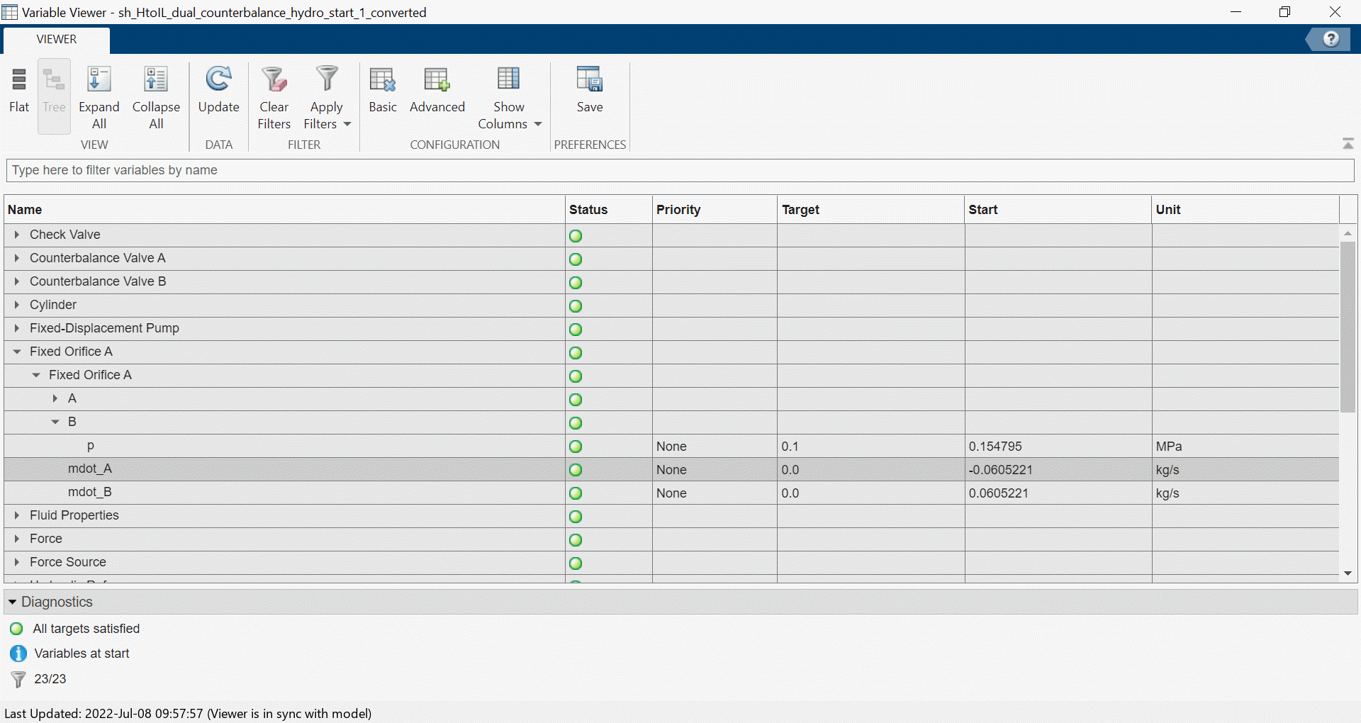
In
sh_HtoIL_dual_counterbalance_hydro_start, open the Variable Viewer. The initial value of the pressure for the Constant Volume Hydraulic Chamber is17010.8 Pa.
Set the converted model to match this value. In the
Pipe Asubsystem ofsh_HtoIL_dual_counterbalance_hydro_start_converted, in theConstant Volume Hydraulic Chamberdialog box, under the Initial targets section, set the Pressure of liquid volume parameter Priority toHighand Value to17010.8 + 101325Pa.Run the converted model. The Variable Viewer shows that the mass flow rate in the
Fixed Orifice Ablock starts at a value of-1.6e-4kg/s. This value is not a perfect match to0kg/s, but it is closer than before.
Interpolation method changed to Linear. Additional elements in the Reynolds number vector, Contraction loss coefficient vector, and Expansion loss coefficient vector may be required.
You can add additional elements to the Reynolds number and loss coefficient vectors in the command line by using the
interp1function.In the hydraulics model, the workspace variable for the Reynolds number vector parameter is defined as
Re_vecand the Loss coefficient vector parameter is defined asloss_coeff_vec. In the MATLAB command window, enter:In theRe_vec_smooth = -6000:100:6000; loss_coeff_vec_smooth = interp1(Re_vec, loss_coeff_vec, Re_vec_smooth, 'makima', 'extrap');
Pipe Asubsystem, replaceRe_vecwithRe_vec_smoothandloss_coeff_vecwithloss_coeff_vec_smoothin theArea Change Bblock dialog:Set the Reynolds number vector parameter to
Re_vec_smooth(Re_vec_smooth>0).Set the Contraction loss coefficient vector parameter to
[interp1( -fliplr(Re_vec_smooth(Re_vec_smooth<0)), fliplr(loss_coeff_vec_smooth(Re_vec_smooth<0)), Re_vec_smooth(Re_vec_smooth>0), 'linear', loss_coeff_vec_smooth(1))].Set the Expansion loss coefficient vector parameter to
loss_coeff_vec_smooth(Re_vec_smooth>0).
The command extrapolates the data set linearly to Re = 6000 and applies a smooth interpolation method the next time the simulation runs.
Only elements greater than or equal to 0 retained in Reynolds number vector. Expansion loss coefficient values mapped to these Reynolds numbers. Adjustment of Reynolds number vector, Contraction loss coefficient vector, and Expansion loss coefficient vector may be required.
The Reynolds number vector in the original
Area Change
                      B
block has both negative and positive Reynolds numbers,[-6000 -4000 -1000 -200 -50 -30 -20 -10 -1 1 20 40 100 500 2000 5000], but the convertedArea Change Bblock only preserves positive Reynolds numbers. The convertedArea Change Bblock in thePipe Asubsystem symmetrically extends the positive elements of the user-provided Reynolds number vector to negative Reynolds numbers. The converted block also separates and extends the loss coefficient vector to individual expansion and contraction loss coefficient vectors. To match the original model behavior, you need to extend the data set to Re = 6000 in the base workspace. The commands in the previous step also addressed this warning.Nominal fluid density and kinematic viscosity removed. Pump uses network fluid properties. Adjustment of Volumetric efficiency at nominal conditions may be required.
In the Hydraulics (Isothermal) library, you can define density and viscosity specifically for pump or motor blocks. Isothermal Liquid blocks use network properties to model these values. To account for this change, adjust the Volumetric efficiency at nominal conditions parameter in the Fixed-Displacement Pump (IL) block:
In the Fixed-Displacement Pump (IL) dialog, set the Volumetric efficiency at nominal conditions parameter to
0.957, which is determined using the formulawhere:
νH,nom is the value of the Nominal kinematic viscosity parameter in the Fixed-Displacement Pump block.
ρH,nom is the value of the Nominal fluid density parameter in the Fixed-Displacement Pump block.
ηH is the value of the Volumetric efficiency at nominal conditions parameter in the Fixed-Displacement Pump block.
νIL is the value of the Kinematic viscosity at atmospheric pressure parameter in the Isothermal Liquid Properties (IL) block.
ρIL is the value of the Density at atmospheric pressure (no entrained air) parameter in the Isothermal Liquid Properties (IL) block.
Save and run
sh_HtoIL_dual_counterbalance_hydro_converted.
To see a model that contains all of the post-conversion updates, open
sh_HtoIL_dual_counterbalance_end, which includes all post-conversion
updates. Inspect the model signals with the Simulation Data Inspector. The Pump Rotational
Velocity signals are now within the tolerance for the majority of the time. There are still
some expected discrepancies when fast dynamics occur.
Conversion for Models That Include Fluid Dynamic Compressibility
Unlike the Hydraulics (Isothermal) library, all blocks in the Isothermal Liquid library account for density as a function of pressure. In some converted models, this can cause diverging results, which this example illustrates.
Open the hydraulic orifice model by entering
ssc_HtoIL_orificeat the command line.Save the model as
ssc_HtoIL_hydro.mdlto a location where you have write permissions.Set the MATLAB Current Folder to this location. The converted model and the conversion report will be saved here.
Run the model.
Convert the blocks in the model to the isothermal liquid library. At the command prompt, enter
hydraulicToIsothermalLiquid('ssc_HtoIL_hydro').Run the converted model.
Open the Simulation Data Inspector and select Compare in the left pane. Set Baseline to
ssc_HtoIL_hydro. Set Compare to tossc_HtoIL_hydro_converted.Click More. Under Global Tolerances set Absolute, Relative, and Time to
0.01.Click Compare.
As the applied pressure increases, the mass flow rates in the Hydraulics (Isothermal) and Isothermal Liquid models diverge.

This divergence is due to the fact that density is constant in the Hydraulics (Isothermal) block and varies as a function of pressure in the Isothermal Liquid block.

Depending on your application, your converted model may require tuning to account for density changes due to changes in pressure or temperature.
See Also
hydraulicToIsothermalLiquid | hydraulicToIsothermalLiquidPostProcess | Simulation Data
Inspector