Data Types in System Identification Toolbox

This example describes different data types and formats supported by System Identification Toolbox.

The toolbox supports model identification using time-domain signals, frequency-domain signals and frequency-response data (also called Frequency Response Function, or FRF). Typically there is no restriction on the number of input and output signals; most estimation commands support an arbitrary number of I/O signals. In particular, there is full support for time-series modeling, or signal modeling, where the data is typically described as having an arbitrary number of outputs, but no inputs.

How Data of Different Types are Generated

The origin of signals is in time-domain where the system or process to be modeled is excited by an external stimulus (the "input" u(t)) and the corresponding response of the system (the "output" y(t)) recorded. These signals are recorded over a finite span of time t resulting in vectors or matrices storing the measured values. The triplet of recorded values $$\{y,u,t\}$$ denoted by $$D_1$$ in the schematic diagram below forms the time-domain data. Since the data can only be recorded at discrete time instants, sometimes an extra piece of information is also required for modeling - the intersample behavior.

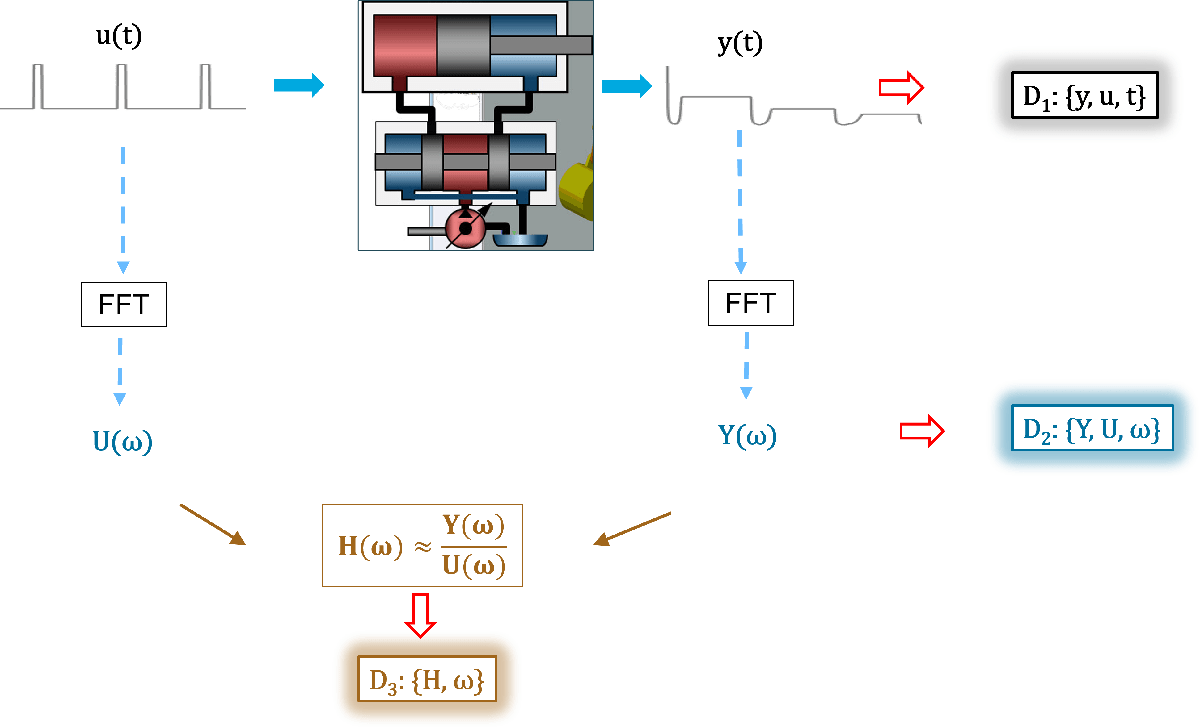
The time-domain signals can be converted into their frequency-domain counterparts by using Discrete Fourier Transform, typically carried out using the FFT operation. This operation requires the time domain signals to be collected on (or interpolated to) a uniform time-grid, that is, made available at a constant sampling interval $$T_s$$. Unless zero-padding is used, the resulting signals correspond to a uniform frequency grid of as many samples as in the original (time-domain) signals and spaced over 0 to Nyquist frequency ($$=\pi /T_s$$, where $$T_s$$ is the time-domain data sampling interval). The triplet$$\{Y,U,\omega \}$$is called frequency-domain data. It is shown by ${\mathit{D}}_2$ in the diagram above. To make the frequency-domain data independent of any correspondence to another time-domain dataset, the sample time $$T_s$$ is also stored.

The dynamic behavior of systems is often described by its frequency response, which is a collection of the gain and relative phase of the output of the system to a sinusoidal input, over a range of input frequencies. Typically spectrum analyzers compute these values. They can also be computed by applying spectral analysis techniques to the time- or frequency-domain data. The result is a complex frequency response vector $$H(\omega )$$ computed over a range of $$\omega$$ values. The pair $$\{H,\omega \}$$is called the frequency response data (FRD) or frequency response function (FRF), shown as ${\mathit{D}}_3$ in the diagram above.

To summarize, System Identification Toolbox supports these 3 data types:

1. Time-domain data: composed of input, output signal values for a given time-vector. The input signal is not always present, such as in case of time-series modeling. Both linear and nonlinear models can be identified using time-domain data.

2. Frequency-domain data: FFT of time-domain signals. Typically used for linear model identification. They offer the benefit of data compression and fast estimation algorithms.

3. Frequency response data (FRD): gain and phase of the system output relative to its input, recorded over a range sinusoidal inputs of varying frequencies. Like frequency-domain data, the FRDs provide the benefit of data compression and fast estimation algorithms. They are used for identifying linear models.

Data Formats: Representation of Various Data Types for Identification Purposes

System Identification Toolbox supports 3 ways of representing time-domain data - time tables, numeric matrices, and iddata objects.

Time Tables

Time tables are a built-in MATLAB datatype represented by the timetable objects. They are used to represent observations that are ordered by time and hence are suitable for time-domain identification. You can create time tables by using the timetable constructor, or by using the array2timetable command. Time tables can be created automatically when importing data into MATLAB from data files (spreadsheets, csv files etc).

The time vector associated with the data in a timetable TT can be accessed using its TT.Properties.RowTimes property. Identification typically requires uniformly sampled data (has a finite value for its "TT.Properties.SampleRate" and "TT.Properties.TimeStep" properties.Time tables are supported for model identification, release R2022b onwards. For earlier releases, you must use iddata object to represent data.

% Example: estimate a continuous-time transfer function using data represented by a timetable
load sdata8 tt8
head(tt8) % view the first few rows of the variables in timetable tt8

      t      u1    u2       u3           y    
    _____    __    __    _________    ________

    1 sec     1     1     -0.62559      1.3563
    2 sec    -1    -1      0.38628      1.2895
    3 sec     1    -1     -0.61745    -0.61873
    4 sec     1     1     -0.72216    -0.10768
    5 sec     1    -1     -0.41638      2.9138
    6 sec     1    -1    -0.002612     0.58144
    7 sec    -1    -1      0.38949     0.20034
    8 sec    -1    -1      -1.1337     -1.0462

np = 2; % number of poles
nz = 2; % number of zeros

% Estimate a model using only one input ('u2') and output ('y')
% (this is just to illustrate a calling syntax; the model quality is not good)
sysTF_a = tfest(tt8, np, nz, 'InputName','u2','OutputName','y');

% Estimate a model with 3 inputs ('u1', 'u2', 'u3') and 1 output ('y')
sysTF_b = tfest(tt8, np, nz, 'InputName',{'u1','u2','u3'},'OutputName','y')

sysTF_b =
 
  From input "u1" to output "y":
  -0.06172 s^2 + 0.1762 s + 1.836
  -------------------------------
      s^2 + 0.3634 s + 0.2453
 
  From input "u2" to output "y":
  1.025 s^2 + 1.679 s + 1.211
  ---------------------------
    s^2 + 0.3707 s + 0.2436
 
  From input "u3" to output "y":
  -0.06868 s^2 - 0.3401 s + 0.5967
  --------------------------------
      s^2 + 0.3603 s + 0.2496
 
Continuous-time identified transfer function.

Parameterization:
   Number of poles: [2 2 2]   Number of zeros: [2 2 2]
   Number of free coefficients: 15
   Use "tfdata", "getpvec", "getcov" for parameters and their uncertainties.

Status:                                   
Estimated using TFEST on time domain data.
Fit to estimation data: 80.91%            
FPE: 1.068, MSE: 0.9817                   
 
Model Properties

Specifying Input Intersample Behavior

An attribute of the input data that is important for continuous-time modeling is its intersample behavior, whether it is held constant between the samples (zero-order-hold), is linear (first-order-hold), or is bandlimited. Specification of this data attribute allows the estimation algorithm to account for potential aliasing effects in the data and deliver the correct result. Use the "InputInterSample" option in the estimation option set to assign the correct value.

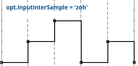
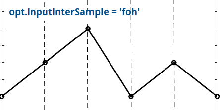
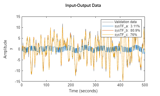
opt = tfestOptions;
opt.InputInterSample = 'foh';
sysTF_c = tfest(tt8, np, nz, 'InputName',{'u1','u2','u3'},'OutputName','y',opt);

% Compare the responses of models sysTF_a, sysTF_b, and sysTF_c to the measured output in tt8
compare(tt8, sysTF_a, sysTF_b, sysTF_c)

Note that the input intersample behavior has no effect on discrete-time estimations.

Multi-Experiment Data

You can use multiple datasets together for model identification. If the data is in timetables, you pass a cell array of the timetables to all the estimation and analysis commands. The individual timetables in the cell array are referred to as "experiments". Thus, the variable X = {TT1, TT2, TT3} represents a multi-experiment dataset consisting of 3 experiments TT1, TT2, and TT3. Each experiment must have the same datatype (timetable here), the same active numeric variables, and the same sample time and time units. The start time, and the number of observations in the individual experiments may be different.

% Load two timetables.
% For the purposes of this example, assume that they both correspond to the same system
% The datasets have different lengths, but are sample at the same rate (10 Hz)
load sdata1 tt1
load sdata2 tt2

% Create a multi-experiment dataset
MultiExpData = {tt1, tt2};

% Estimate a nonlinear ARX model using MultiExpData
Orders = [5 5 1];
NL = idGaussianProcess;
nlsys = nlarx(MultiExpData, Orders, NL)

nlsys =

Nonlinear ARX model with 1 output and 1 input
  Inputs: u
  Outputs: y

Regressors:
  Linear regressors in variables y, u
  List of all regressors

Output function: Gaussian process function using a SquaredExponential kernel
Sample time: 0.1 seconds

Status:                                                  
Estimated using NLARX on time domain data "MultiExpData".
Fit to estimation data: [79.04 87.04]% (prediction focus)
FPE: 0.9208, MSE: [0.8527 0.8901]                        

Model Properties

% Compare the model response to the estimation data
%compare(MultiExpData, nlsys)

The plot shows the fit to the first dataset. Right-click on the plot and use the context menu to pick the second data experiment to view.

% Example: perform spectral analysis on the multi-experiment data, that is, estimate the frequency
% response
G = spa(MultiExpData);
bode(G)

Relationship of Time Tables to the IDDATA object

The timetable object is a basic datatype available in MATLAB and is the recommended way of representing time-domain signals. The iddata object is specific to System Identification Toolbox. It can be used to store both time-domain signals as well frequency-domain signals.

Numeric Matrices

The model training, validation, and analysis commands accept numeric matrices for the input and output data. The observations are along the rows and the channels are along the columns. This is the simplest data format and is often sufficient for identifying discrete-time models. Note that this format does not provide any information about the time vector. Hence this format is not recommended for identifying continuous-time models.

% load double matrices
% umat1: input vector, ymat1: output vector
load sdata1 umat1 ymat1
% Estimate a discrete-time state-space model of 4th order
sysd = n4sid(umat1, ymat1, 4)

sysd =
  Discrete-time identified state-space model:
    x(t+Ts) = A x(t) + B u(t) + K e(t)
       y(t) = C x(t) + D u(t) + e(t)
 
  A = 
              x1         x2         x3         x4
   x1     0.8392    -0.3129    0.02105    0.03743
   x2     0.4768     0.6671     0.1428   0.003757
   x3   -0.01951    0.08374   -0.09761      1.046
   x4  -0.003885   -0.02914    -0.8796   -0.03171
 
  B = 
              u1
   x1    0.02635
   x2   -0.03301
   x3  7.256e-05
   x4  0.0005861
 
  C = 
            x1       x2       x3       x4
   y1    69.08    26.64   -2.237  -0.5601
 
  D = 
       u1
   y1   0
 
  K = 
              y1
   x1   0.003282
   x2   0.009339
   x3  -0.003232
   x4   0.003809
 
Sample time: 1 seconds

Parameterization:
   FREE form (all coefficients in A, B, C free).
   Feedthrough: none
   Disturbance component: estimate
   Number of free coefficients: 28
   Use "idssdata", "getpvec", "getcov" for parameters and their uncertainties.

Status:                                           
Estimated using N4SID on time domain data "umat1".
Fit to estimation data: 76.33% (prediction focus) 
FPE: 1.21, MSE: 1.087                             
 
Model Properties

sysd.Ts

ans = 1

Since the data does not provide the sample time, it is assumed to be 1 second. Consequently, the model sample time, sysd.Ts, is also 1 second (note that n4sid estimates a discrete-time model by default). Since the data does not provide the sample time information, you can choose a different sample time for the model by using the'Ts'/<value> name-value pair.

% Estimate a discrete-time state-space model of sample time 0.1 seconds
sysd = n4sid(umat1, ymat1, 4, 'Ts', 0.1);

In the above call, the sample time (Ts) of the model is assigned a value of 0.1 seconds. In order to achieve this, the data sample time is also assumed to be 0.1 seconds. This simple assignment of the sample time does not work if a continuous-time model is desired.

% Estimate a continuous-time state-space model 
sysc = n4sid(umat1, ymat1, 4, 'Ts', 0);

Warning: Data sample time is assumed to be 1 seconds. To specify a different value for the data sample time consider providing data using a timetable or an iddata object.

In this case, there is no direct way of specifying the data sample time; it is assumed to be 1 second. The warning issued is pointing to this fact. If you have the data in numeric format, convert it into a timetable or an iddata object wherein you can add the information regarding the sampling (such as the value of sample time and the time unit). Suppose the true sample time of the data above is 0.1 hours. In order to pass this formation to N4SID, you can proceed as follows.

N = size(umat1,1);
% (assume a start time of 1 hr)
t = hours(0.1*(1:N)');
dataTT = timetable(umat1,ymat1,'RowTimes',t);
sysc = n4sid(dataTT, 4, 'Ts', 0);
sysc.Ts

ans = 0

sysc.TimeUnit

ans = 
'hours'

You can, alternatively, use an iddata object to represent the data.

dataIDDATA = iddata(ymat1, umat1, 0.1, 'TimeUnit', 'hours');
sysc = n4sid(dataIDDATA, 4, 'Ts', 0);
sysc.Ts

ans = 0

sysc.TimeUnit

ans = 
'hours'

The IDDATA Object

Convert Data Between Time and Frequency Domains

Time-Series and Signal Modeling