Visualize Point Clouds on Maps Using Coordinate Reference System from LAS/LAZ Files
This example shows how to use coordinate reference system (CRS) information in LAS/LAZ files to transform a point cloud from one coordinate reference system to another. Converting two point clouds collected at the same geographic location but stored in different reference systems is important for data analysis, combining multiple point clouds and comparison.
A CRS defines point cloud coordinates in real-world locations. Two common types of CRSs are:
Projected: Assigns cartesian x and y map coordinates to physical locations.
Geographic: Assigns latitude, longitude, height to physical locations.
Projected CRSs consist of a geographic CRS and several parameters that are used to transform coordinates to and from the geographic coordinates. Point clouds can also be transformed from one projected CRS to another. To learn more about CRS, see Transform Coordinates to a Different Projected CRS and Project and Display Raster Data examples.
A LAS/LAZ file contains CRS information, specified by American Society for Photogrammetry and Remote Sensing (ASPRS), enabling to transform coordinates of point clouds stored in them.
Load Point Cloud
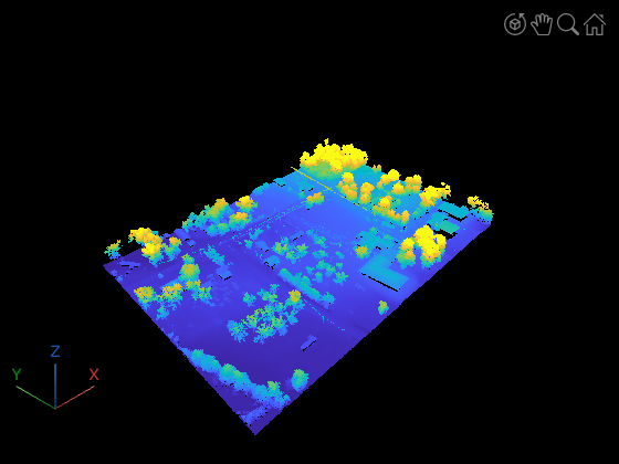
Read point cloud from a LAZ file for an area near Tuscaloosa, Alabama [1].
% Load point cloud from a LAZ file
fileName = fullfile(toolboxdir("lidar"),"lidardata","las","aerialLidarData.laz");
lasReader = lasFileReader(fileName);
ptCloud = readPointCloud(lasReader);

% Visualize
pcviewer(ptCloud);
Read Coordinate System Information
Read projected CRS information from the LAZ file using readCRS function. A projected CRS consists of a geographic CRS and several parameters that are used to transform coordinates between Cartesian and geographic coordinates.
crs = readCRS(lasReader)
crs =
  projcrs with properties:

                    Name: "NAD83 / UTM zone 16N"
           GeographicCRS: [1×1 geocrs]
        ProjectionMethod: "Transverse Mercator"
              LengthUnit: "meter"
    ProjectionParameters: [1×1 map.crs.ProjectionParameters]
To know more about this reference system, visit the Spatial Reference home page. Click on List all references and search for "NAD83 / UTM zone 16N". You will find one reference system that exactly matches this name, identified by the code EPSG:26916. Click on it for more information. This reference system covers parts of North America, including state of Alabama.
Each geographic region is associated with one or more reference systems, each identified by a projected CRS code published by the EPSG organization. You can also find this information in a projcrs (Mapping Toolbox) object by using the output of wktstring (Mapping Toolbox) function. See the end of the output string to obtain the code.
Visualize Area of Data Acquisition
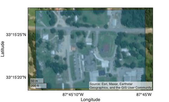
CRS information can be used to visualize on a map, the area from which the point cloud was acquired. This is helpful for performing geospatial analysis and working with other data sources for the same area, such as, satellite imagery.
% Define an Area of Interest (AOI)
xLimits = ptCloud.XLimits;
yLimits = ptCloud.YLimits;
aoi = aoiquad(xLimits,yLimits,crs);

% Visualize AOI overlaid on a map
figure
geobasemap satellite
geoplot(aoi)
Visualize Point Cloud on 3-D Globe
CRS information can be used to plot a point cloud on a geographic globe. This map visualization aids in verifying data acquisition and is also useful for assessing map-building algorithms such as SLAM.
% Convert x-y coordinates to latitude-longitude.
[lat, lon] = projinv(crs,ptCloud.Location(:,1),ptCloud.Location(:,2));

% Use z-coordinate as height
height = ptCloud.Location(:,3);

% Visualize
fig = uifigure;
globe = geoglobe(fig);
gplot = geoplot3(globe,lat,lon,height,"o",MarkerSize=2);

% Adjust graphics camera position to bring it closer to the
% point cloud for better visibility.
campos(globe, 33.25475, -87.75359,  89.24658)
camheight(globe, 89.2466)
camheading(globe, 356.3342)
campitch(globe, -17.8413)
camroll(globe, 360)
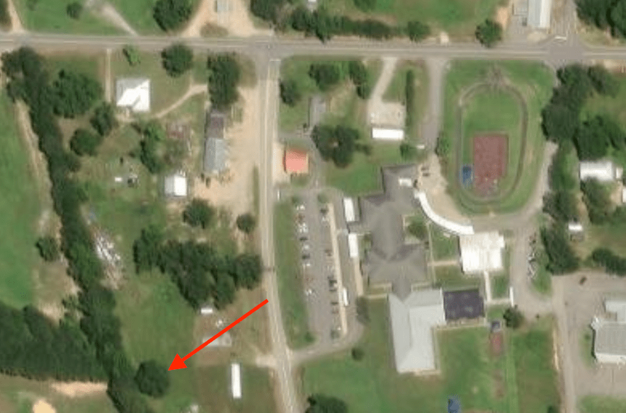
The tree indicated by the arrow in the above image is represented in point cloud on the map in the image below. To tilt and rotate the globe, hold the Ctrl key and drag.
im = getframe(fig);
figure; imshow(im.cdata, Border="tight");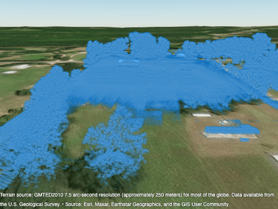
Working with Geographic CRS
Point clouds can also be stored in geographic coordinates in a LAS/LAZ file. In this case, readCRS function returns a geocrs (Mapping Toolbox) object. Read a point cloud from the same location in Tuscaloosa, Alabama, stored in geographic coordinates (latitude and longitude).
% Load point cloud
geolasreader = lasFileReader("aerialLidarDataGeo.laz");
Warning: File contains data referenced to geographic coordinates, but point cloud functions expect data referenced to Cartesian coordinates. To convert, see the "Working with Geographic CRS" section in the <a href="matlab:helpview('lidar','CoordinateReferenceSystemInLASFilesExample') ">Visualize Point Clouds On Maps Using Coordinate Reference System From LAS/LAZ Files</a> example.
Each point in this point cloud is from the same geographic location as the points in aerialLidarData.laz. Location property of the point cloud object stores latitude, longitude and height in three dimensions respectively.
% Display point cloud.
geoPtCloud = readPointCloud(geolasreader)
geoPtCloud =
pointCloud with properties:
Location: [1018047×3 double]
Count: 1018047
XLimits: [-87.7543 -87.7499]
YLimits: [33.2552 33.2578]
ZLimits: [72.7900 125.8200]
Color: []
Normal: []
Intensity: [1018047×1 uint16]
% Read geographic CRS.
crsGeo = readCRS(geolasreader)
crsGeo =
geocrs with properties:
Name: "NAD83"
Datum: "North American Datum 1983"
Spheroid: [1×1 referenceEllipsoid]
PrimeMeridian: 0
AngleUnit: "degree"
From the CRS name and the Spatial Reference home page, it is evident that the coordinate system used here is the North American Datum of 1983 (NAD83). Another common geographic CRS found in LAS/LAZ files is the World Geodetic System of 1984 (WGS84), a global reference system used by GPS and widely adopted in mapping and navigation.
Incorrect Visualization with Geographic Coordinates
Point cloud functions and apps require Cartesian coordinates to visualize and process point clouds. For this point cloud, the pcshow and pcviewer functions incorrectly visualize the data because the latitude-longitude coordinates cover a small range of values.
figure
pcshow(geoPtCloud)
title("Incorrect Visualization")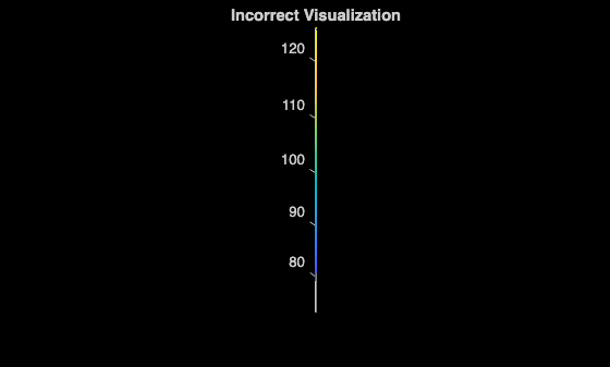
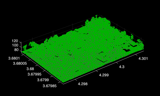
When the latitude-longitude coordinates cover a small range of values, you can improve the visualization by changing the data aspect ratio of the axes object. Preview the point cloud by using the daspect function to make each 1 unit in the x-axis (longitude) and y-axis (latitude) directions equal to 100,000 units in the z-axis direction. To process and accurately visualize the point cloud data, you must convert the data to Cartesian coordinates. If you choose to work in geographic coordinates, then your measurements will be distorted because of Earth's curvature.
h = pcshow(geoPtCloud);
daspect(h,[1 1 100000])
title("Modified Aspect Ratio")
xlabel("Longitude")
ylabel("Latitude")
zlabel("Height")

Convert to Cartesian Coordinates
To visualize or process this point cloud, convert the geographic coordinates to Cartesian coordinates. Projected CRS information is necessary for this conversion. In the absence of this information, it can be obtained from the Spatial Reference home page by following these steps:
Click on Explorer and select a location of interest on the map, in this case, Tuscaloosa, Alabama.
Select Projected and EPSG checkbox.
Enter "
NAD83" in the Filter by name field.Choose one of the systems listed.
EPSG:26916 was selected because it matches the code from the original LAZ file, as this information is already known. Create a projcrs (Mapping Toolbox) object.
proj = projcrs(26916)
proj =
  projcrs with properties:

                    Name: "NAD83 / UTM zone 16N"
           GeographicCRS: [1×1 geocrs]
        ProjectionMethod: "Transverse Mercator"
              LengthUnit: "meter"
    ProjectionParameters: [1×1 map.crs.ProjectionParameters]
Verify if it has the same geographic CRS.
disp(proj.GeographicCRS)
  geocrs with properties:

             Name: "NAD83"
            Datum: "North American Datum 1983"
         Spheroid: [1×1 referenceEllipsoid]
    PrimeMeridian: 0
        AngleUnit: "degree"
disp(crsGeo)
  geocrs with properties:

             Name: "NAD83"
            Datum: "North American Datum 1983"
         Spheroid: [1×1 referenceEllipsoid]
    PrimeMeridian: 0
        AngleUnit: "degree"
Project latitude-longitude coordinates to x-y coordinates using projfwd (Mapping Toolbox) function, and use the height from the point cloud object as the z-coordinate.
[x, y] = projfwd(proj, geoPtCloud.Location(:,2), geoPtCloud.Location(:,1));
z = geoPtCloud.Location(:,3);
tformedPtCloud = pointCloud([x y z]);
Visualize the point cloud converted to Cartesian coordinates.
pcviewer(tformedPtCloud);
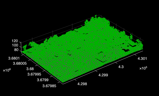
To verify the conversion from geographic coordinates to Cartesian, you can compare the point cloud from aerialLidarData.laz which is stored in Cartesian coordinates and tformedPtCloud, which is a converted point cloud from geographic to Cartesian coordinated. Visualizing the two point clouds in pcshowpair, shows that there is no difference between them, verifying the accuracy of the conversion. If there was a difference, the point clouds would be misaligned and colored magenta and green respectively.
figure
pcshowpair(ptCloud, tformedPtCloud)
References
[1] OpenTopography. Tuscaloosa, AL: Seasonal Inundation Dynamics And Invertebrate Communities. OpenTopography, 2011. DOI.org (Datacite), https://doi.org/10.5069/G9SF2T3K