Set Up Sum Optimizations

CAGE can solve sum-type optimizations. These optimizations find the optimal settings of control parameters at several operating points simultaneously. You can use sum optimizations to solve drive-cycle problems where you must apply the constraints across the whole cycle, for example, a constraint such as weighted engine out brake-specific NOx <= 3 g/kWh.

If you have an existing point optimization, you can use a utility to create a sum optimization from your point optimization output. This approach can help you find good initial values for a sum optimization. To create a sum optimization from your point optimization:

• (Recommended) Select Solution > Create Sum Optimization. For more details, see Create Sum Optimization from Point Optimization Output.

• Select Optimization > Convert to Sum Optimization.

If you do not have an existing point optimization, set up a new sum optimization using the Optimization Quick Start Tool. To configure a sum objective in the tool, specify objectives, constraints, and operating points. CAGE automatically configures your variable values correctly for a sum optimization, which defines a single run. Use scalar variables when an optimization variable is the same for all operating points. You can only use table gradient constraints and sum constraints in sum optimizations. Optionally, you can evaluate objectives or constraints over different operating points than those you specified in the optimization. See Using Application Point Sets. For descriptions of optimization output specific to sum problems, see Interpret Sum Optimization Output.

Using Application Point Sets

You can use application point sets to evaluate constraints and objectives at different operating points than those specified in the optimization. You can only use application point sets with sum optimizations.

Application point sets can be useful for problems such as these:

• Your calibration problem requires consideration of several drive cycles, defined at different operating point sets. For example, problems often have different drive cycles for performance and emissions.

• You want to apply some constraints only at a subset of the optimization points (sometimes called multiregion problems). For example, you must often consider different constraints at full load.

• Your full operating point set of interest is large and optimizing at every point is slow. You can run an optimization at a subset of points, and evaluate interpolated results across an application point set.

• You need to evaluate point-by-point models at different operating points to the points where the models are defined.

To use an application point set for evaluating an objective or constraint:

1. Right-click the objective or constraint, and select Select Application Point Set.

   The Select Operating Point Variables dialog box appears.

2. Select a pair of variables to use in application point sets. The variables must be fixed variables in your optimization. You only select variables once per optimization. Click OK.

   The Select Application Point Set dialog box appears.

3. Select an application point set. You can choose a data set or a New subset of the optimization points. To select a subset of points, you can use the check boxes or click points on the plot.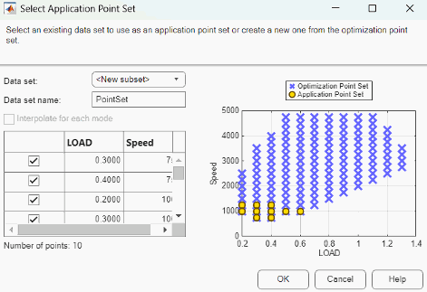

   

4. View the plot displaying the application points and optimization points. CAGE extrapolates the optimization results to evaluate the objective or constraint at the application points.

5. Click OK.

To see example plots that illustrate how CAGE uses application point sets, enter mbcAppPointSetDemo, which loads the example project file mbcAppPointSetDemo.cag into CAGE. Run the optimizations in the project to view the plots.

Selecting Scalar Variables

At the optimization node, the Optimization Point Set pane lists the free and fixed variables. For sum optimizations:

• The Number of operating points value is the number of points that the optimizer sums during the optimization.

• Set Select Scalar Variables to specify the scalar values that do not depend on the operating points.

Example Problem to Demonstrate Controls for Sum Optimizations

The following sections describe the controls and outputs for sum optimizations using the following example problem for illustration.

Say you have created models for torque (TQ), residual fraction (RESIDFRAC) and exhaust temperature (EXTEMP) for a gasoline engine.

The inputs to these models are:

• Spark advance, S

• Intake cam timing, INT

• Exhaust cam timing, EXH

• Engine speed, N

• Relative load, L

You need to set up an optimization to calculate optimal settings of S, INT and EXH for the operating points shown in the table.

N	L
1000	0.3
1100	0.2
1250	0.31
1500	0.25
1625	0.18

The objective for this optimization is to maximize the weighted sum of TQ over the operating points.

The constraints for this optimization are:

• Constraint 1: EXTEMP <= 1290°C at each operating point

• Constraint 2: RESIDFRAC <= 17% at each operating point

• Constraint 3: Change in INT is no more than 5.5° per 500 rpm change in N and 5.5° per 0.1 change in L, evaluated over a 3-by-3 (N, L) table.

• Constraint 4: Change in EXH is no more than 5.5° per 500 rpm change in N and 5.5° per 0.1 change in L, evaluated over a 3-by-3 (N, L) table.

You can use the fmincon algorithm in CAGE to solve this problem.

This example is used to explain the controls and outputs in the following sections, Selecting Scalar Variables and Interpret Sum Optimization Output.

For details on the optimization algorithm restrictions in CAGE, see Applying Constraints to Operating Points.

Applying Constraints to Operating Points

Each solver needs to evaluate the objectives and constraints to determine the optimal solution. Optimization solvers typically have restrictions on the number of objective and constraint outputs they can handle. The following tables show how CAGE applies constraints over multiple operating points for point and sum optimizations.

Optimization Type	Objectives
Single-objective	One output
Multiobjective	Two or more outputs

Use point objectives for point optimizations, and use sum objectives for sum optimizations. You can also use sum objectives for point optimizations: the optimization sums a single objective value with weights. You cannot use point objectives for sum optimizations.

CAGE sets up the sum objective correctly when creating the optimization or converting to a sum. CAGE defaults to a sum objective when adding an objective to a multiobjective sum.

This table details the number of outputs each objective type returns as a function of the maximum number of values of all of its inputs. N is the number of operating points.

Objective Type	Maximum Number of Values of All Inputs to the Objective	Number of Outputs	Description
Point	N	N	A point objective is evaluated at each operating point within a run, and all the values are returned.
Sum	N	1	A sum objective evaluates a model at every operating point and returns one value, which is the weighted sum of the model evaluations.

This table details the number of outputs each constraint type returns as a function of the maximum number of values of all of its inputs.

Constraint Type	Number of Constraints Output	Description
Linear	1 at each operating point	These constraints are evaluated at every operating point within a run, and all values are returned.
Ellipsoid	1 at each operating point
1D Table	1 at each operating point
2D Table	1 at each operating point
Model	1 at each operating point
Range	1 or 2 at each operating point	A range constraint evaluates an expression at each operating point within a run. The constraint returns two values for each point: the distance from the lower bound, and the distance from the upper bound. In this case, 2N outputs are returned. If one of the bounds is infinite, then only the distance to the finite bound is returned for each point, and N outputs are returned. If both bounds are infinite, then 0 outputs are returned.
Sum	1	A sum constraint evaluates a model at every operating point and returns the difference between the weighted sum of the model and a bound.
Table	2((n-1))m + (m-1)n for 2D 2(n-1)for 1D	A table gradient constraint constrains the gradient of an optimization variable over a grid. The number of outputs returned depends on the dimensions of the grid. Any infinite bound [0, Inf] means strictly increasing, and results in half the number of constraints.

You can use the tables in this section to check whether the problem setup satisfies the algorithm restrictions. As an example, the next table shows how to check whether the example problem in Example Problem to Demonstrate Controls for Sum Optimizations satisfies the restriction of the algorithm chosen to solve it, fmincon.

Objective	Maximum Number of Values of All Inputs	Number of Outputs
Weighted sum of TQ over the drive cycle points	5	1 (using the Objective table)

Constraint	Maximum Number of Values of All Inputs	Number of Outputs
EXTEMP <= 1290°C at each drive cycle point	5	5 (using the Constraint table)
RESIDFRAC <= 17% at each drive cycle point	5	5 (using the Constraint table)
Change in INT is no more than 5.5° per 500 rpm and 5.5° per 0.1 change in L	5	24 (this value is the number of table gradient constraint outputs generated from a 3-by-3 table)
Change in EXH is no more than 5.5° per 500 rpm and 5.5° per 0.1 change in L	5	24 (this value is the number of table gradient constraint outputs generated from a 3-by-3 table)

Thus, the example problem has one objective output and 58 constraint outputs. This output satisfies the restrictions of the fmincon solver, so the algorithm can be used.