Simulate Nonisolated Converter Voltage Mode Control

R2026b

This example uses:

This example shows how to design and simulate voltage mode control for three nonisolated DC-DC converter topologies using Motor Control Blockset(TM). You compare open-loop operation, where the duty cycle is fixed at a precalculated steady-state value, against closed-loop operation, where a PI controller actively regulates the output voltage.

In this example, you:

Compare open-loop and closed-loop Buck converter responses for a 12 V to 6 V step-down application
Compare open-loop and closed-loop Boost converter responses for a 12 V to 20 V step-up application
Compare open-loop and closed-loop Buck-Boost converter responses for a 16 V to 12 V inverting application
Compare closed-loop output voltage step responses across all three topologies

Open and Simulate the Buck Converter

Voltage mode control regulates the converter output voltage by comparing it to a reference and adjusting the pulse-width modulation (PWM) duty cycle through a PI controller. The Buck converter steps voltage down, so the steady-state duty cycle is $D = V_{o u t} / V_{i n}$ . For this model, $V_{i n} = 12 V$ and $V_{o u t, r e f} = 6 V$ , giving an open-loop duty cycle of 0.5.

Open the prebuilt model. The model loads the plant and controller parameters into the workspace using the script BuckVoltageControllerData. This script sets the inductance L, capacitance C, switching frequency Fsw, and the control sample time Tsc that the DCDC Controller Parameters block uses to compute the PI gains for the closed-loop controller.

open_system("BuckVoltageControl")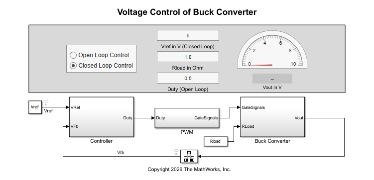

The model contains a Buck Converter subsystem built with Simscape™ Electrical™ blocks, a Controller subsystem with the DCDC Controller Parameters block and the DCDC Voltage Controller block, and a PWM subsystem. The DCDC Controller Parameters block computes PI gains from the plant parameters in the workspace as described in the previous section. In the Controller subsystem, the OL_CL_Switch block selects between open-loop and closed-loop operation based on the LoopSelect constant: set it to 0 for a fixed duty cycle or 1 for PI control. The following image shows the plant topology used in this model.

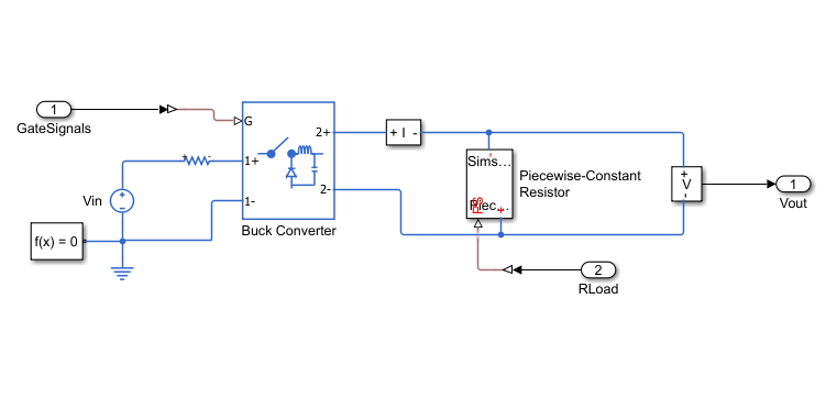
To observe the unregulated Buck converter response, simulate in open-loop mode. In open-loop, the duty cycle is fixed at DutyOpen = Vref/Vin = 0.5, the nominal steady-state value computed by the data script.

set_param("BuckVoltageControl/Controller/LoopSelect", Value="0")
sim("BuckVoltageControl");
buckOLRunIDs = Simulink.sdi.getAllRunIDs();
buckOLRun = Simulink.sdi.getRun(buckOLRunIDs(end));
buckOLVfbID = buckOLRun.getSignalIDsByName("Vfb");
buckOLVfb = buckOLRun.getSignal(buckOLVfbID(1)).Values;

In open-loop, the output voltage settles to a value determined by the fixed duty cycle and load resistance alone. There is no error-correction mechanism. If the load or input voltage deviates from the design point, the output drifts without recovery.

To activate the PI controller and simulate closed-loop voltage regulation, set LoopSelect to 1. The DCDC Voltage Controller block now computes the duty cycle from the error between Vref and Vfb at each control sample step of 50 µs.

set_param("BuckVoltageControl/Controller/LoopSelect", Value="1")
sim("BuckVoltageControl");
buckCLRunIDs = Simulink.sdi.getAllRunIDs();
buckCLRun = Simulink.sdi.getRun(buckCLRunIDs(end));
buckCLVfbID = buckCLRun.getSignalIDsByName("Vfb");
buckCLVfb = buckCLRun.getSignal(buckCLVfbID(1)).Values;

To compare the open-loop and closed-loop responses, plot both Vfb signals on the same axes.

figure
plot(buckOLVfb.Time, buckOLVfb.Data)
hold on
plot(buckCLVfb.Time, buckCLVfb.Data)
yline(6, "--", "V_{ref} = 6 V", LabelHorizontalAlignment="left")
xlabel("Time (s)")
ylabel("Output Voltage (V)")
title("Buck Converter: Open-Loop vs Closed-Loop")
legend("Open-Loop", "Closed-Loop", Location="southeast")
grid on

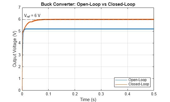
Figure contains an axes object. The axes object with title Buck Converter: Open-Loop vs Closed-Loop, xlabel Time (s), ylabel Output Voltage (V) contains 3 objects of type line, constantline. These objects represent Open-Loop, Closed-Loop.

At the nominal design point, both responses settle near 6 V because the simulation uses the exact plant parameters the data script assumes. The key advantage of closed-loop control becomes apparent when operating conditions shift: the open-loop duty cycle stays fixed at 0.5 while the closed-loop controller adjusts the duty cycle to drive the error to zero. The closed-loop response settles near 5.98 V with a small overshoot to approximately 6.07 V.

Open and Simulate the Boost Converter

The Boost converter steps voltage up with steady-state duty cycle $D = 1 - V_{i n} / V_{o u t}$ . For this model, $V_{i n} = 12 V$ and $V_{o u t, r e f} = 20 V$ , giving an open-loop duty cycle of 0.4. The Boost converter has a right-half-plane (RHP) zero in its control-to-output transfer function, which limits the achievable closed-loop bandwidth. When the DCDC Controller Parameters block computes gains with ConvType set to Boost, it accounts for the RHP zero and returns a more conservative Kp and Ki than it would for a Buck converter with the same plant.

Open the prebuilt Boost converter model. To load the Boost converter parameters, the models calls the Boost data script BoostVoltageControlData. This script sets L = 250 µH, C = 1000 µF, Fsw = 100 kHz, and the control sample time.

open_system("BoostVoltageControl")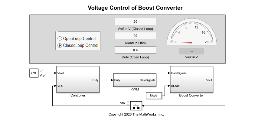

The following image shows the plant topology used in this model.

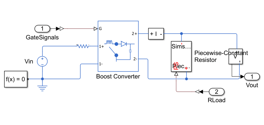
This model uses a variable-step solver to handle the switching dynamics at 100 kHz. The larger capacitance of 1000 µF reduces output voltage ripple but increases the RC time constant and slows settling relative to the Buck converter.

To simulate the open-loop Boost converter response, set LoopSelect to 0. In open-loop, the duty cycle is fixed at DutyOpen = 1 - Vin/Vref = 0.4.

set_param("BoostVoltageControl/Controller/LoopSelect", Value="0")
sim("BoostVoltageControl");
boostOLRunIDs = Simulink.sdi.getAllRunIDs();
boostOLRun = Simulink.sdi.getRun(boostOLRunIDs(end));
boostOLVfbID = boostOLRun.getSignalIDsByName("Vfb");
boostOLVfb = boostOLRun.getSignal(boostOLVfbID(1)).Values;

In open-loop, the Boost converter output settles at the voltage determined by the fixed duty cycle and load. The RHP zero means that a sudden increase in duty cycle causes the output voltage to initially drop before it rises. The PI controller must account for this effect by keeping the closed-loop bandwidth well below the RHP zero frequency.

To simulate closed-loop Boost converter regulation, set LoopSelect to 1.

set_param("BoostVoltageControl/Controller/LoopSelect", Value="1")
sim("BoostVoltageControl");
boostCLRunIDs = Simulink.sdi.getAllRunIDs();
boostCLRun = Simulink.sdi.getRun(boostCLRunIDs(end));
boostCLVfbID = boostCLRun.getSignalIDsByName("Vfb");
boostCLVfb = boostCLRun.getSignal(boostCLVfbID(1)).Values;

To compare the open-loop and closed-loop Boost converter responses, plot both Vfb signals.

figure
plot(boostOLVfb.Time, boostOLVfb.Data)
hold on
plot(boostCLVfb.Time, boostCLVfb.Data)
yline(20, "--", "V_{ref} = 20 V", LabelHorizontalAlignment="left")
xlabel("Time (s)")
ylabel("Output Voltage (V)")
title("Boost Converter: Open-Loop vs Closed-Loop")
legend("Open-Loop", "Closed-Loop", Location="southeast")
grid on

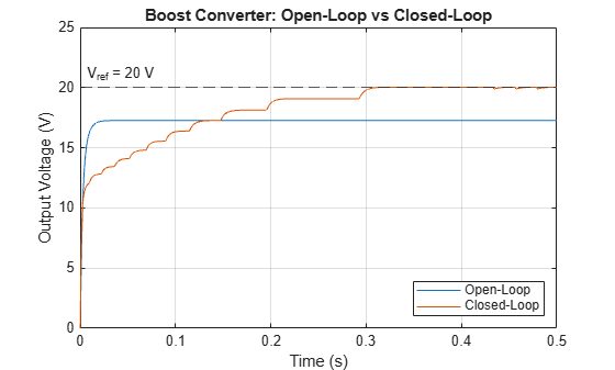
Figure contains an axes object. The axes object with title Boost Converter: Open-Loop vs Closed-Loop, xlabel Time (s), ylabel Output Voltage (V) contains 3 objects of type line, constantline. These objects represent Open-Loop, Closed-Loop.

The closed-loop response rises to approximately 19.95 V and holds near the 20 V reference. At the nominal design point, the open-loop response also reaches 20 V, but without feedback any deviation in load or input voltage causes uncompensated error. The gains chosen by the DCDC Controller Parameters block are intentionally conservative for this topology. The RHP zero constrains how aggressively the integrator can drive the error to zero before introducing oscillations.

Open and Simulate the Buck-Boost Converter

The Buck-Boost converter produces an output voltage of opposite polarity to the input with steady-state duty cycle $D = V_{o u t} / (V_{i n} + V_{o u t})$ . For this model, $V_{i n} = 16 V$ and $V_{o u t, r e f} = 12 V$ , giving an open-loop duty cycle of approximately 0.43. Like the Boost topology, the Buck-Boost has an RHP zero, and its inverting nature produces a characteristic negative transient during startup. Setting ConvType to Buck-Boost on the DCDC Controller Parameters block selects a compensator design that accounts for both the RHP zero and the polarity inversion.

Open the prebuilt Buck-Boost converter model. To load the Buck-Boost converter parameters, the model calls the Buck-Boost data script BuckBoostVoltageControlData. This script sets L = 200 µH, C = 4700 µF, Fsw = 200 kHz, and the control sample time.

open_system("BuckBoostVoltageControl")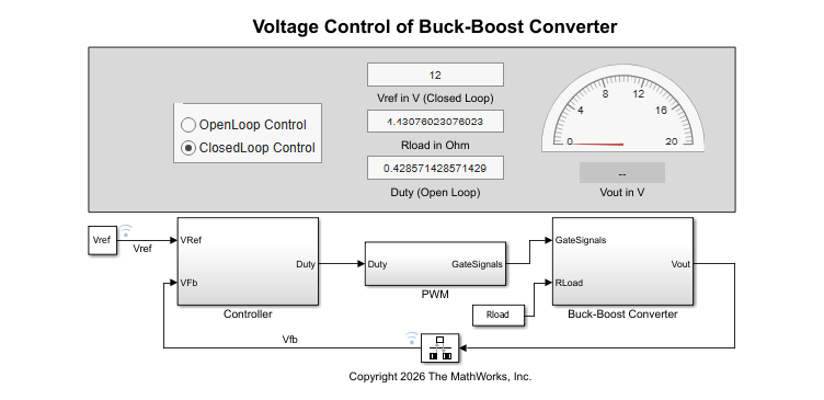

The following image shows the plant topology used in this model.

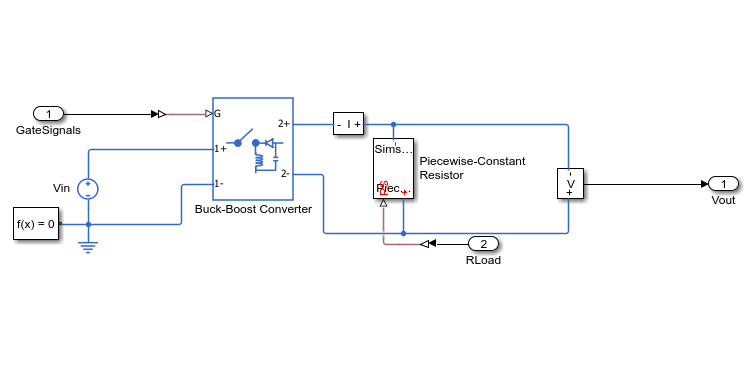
This model uses a fixed-step discrete solver with a step size of 0.5 µs (Ts = 1/(10*Fsw)) to resolve the 200 kHz switching frequency. The capacitance of 4700 µF is much larger than in the other topologies, which increases the charge time and slows the output voltage rise toward the reference.

To simulate the open-loop Buck-Boost response, set LoopSelect to 0. In open-loop, the duty cycle is fixed at DutyOpen = Vref/(Vin + Vref).

set_param("BuckBoostVoltageControl/Controller/LoopSelect", Value="0")
sim("BuckBoostVoltageControl");
bbOLRunIDs = Simulink.sdi.getAllRunIDs();
bbOLRun = Simulink.sdi.getRun(bbOLRunIDs(end));
bbOLVfbID = bbOLRun.getSignalIDsByName("Vfb");
bbOLVfb = bbOLRun.getSignal(bbOLVfbID(1)).Values;

In open-loop, the inverting topology produces a negative initial transient before the output climbs toward steady state. This is normal for the Buck-Boost converter: the inductor stores energy from the input before transferring it to the output capacitor, causing the output to swing negative initially. Without feedback, the output settles at the value determined by DutyOpen and the load.

To simulate closed-loop Buck-Boost regulation, set LoopSelect to 1.

set_param("BuckBoostVoltageControl/Controller/LoopSelect", Value="1")
sim("BuckBoostVoltageControl");
bbCLRunIDs = Simulink.sdi.getAllRunIDs();
bbCLRun = Simulink.sdi.getRun(bbCLRunIDs(end));
bbCLVfbID = bbCLRun.getSignalIDsByName("Vfb");
bbCLVfb = bbCLRun.getSignal(bbCLVfbID(1)).Values;

To compare the open-loop and closed-loop Buck-Boost converter responses, plot both Vfb signals.

figure
plot(bbOLVfb.Time, bbOLVfb.Data)
hold on
plot(bbCLVfb.Time, bbCLVfb.Data)
yline(12, "--", "V_{ref} = 12 V", LabelHorizontalAlignment="left")
xlabel("Time (s)")
ylabel("Output Voltage (V)")
title("Buck-Boost Converter: Open-Loop vs Closed-Loop")
legend("Open-Loop", "Closed-Loop", Location="southeast")
grid on

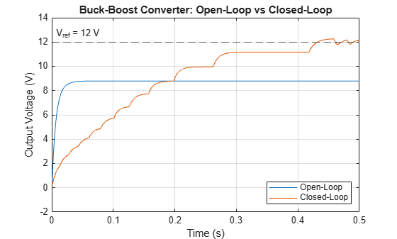
Figure contains an axes object. The axes object with title Buck-Boost Converter: Open-Loop vs Closed-Loop, xlabel Time (s), ylabel Output Voltage (V) contains 3 objects of type line, constantline. These objects represent Open-Loop, Closed-Loop.

Both responses exhibit the negative initial transient characteristic of the inverting topology. The closed-loop controller converges toward 12 V by the end of the simulation, while the open-loop response settles at the fixed operating point. The large 4700 µF capacitor slows both responses.

Compare the Closed-Loop Converter Voltage Responses

Plotting the three closed-loop output voltage waveforms together shows how topology, component values, and operating point each affect the closed-loop response. Because the DCDC Controller Parameters block computes gains from each plant description separately, the three controllers use different PI gains internally. As a result, any differences in settling time, overshoot, and transient shape reflect both the plant dynamics and the topology-appropriate compensator the block selects.

figure
subplot(3,1,1)
plot(buckCLVfb.Time, buckCLVfb.Data)
yline(6, "--")
ylabel("V_{out} (V)")
title("Buck: V_{ref} = 6 V")
grid on

subplot(3,1,2)
plot(boostCLVfb.Time, boostCLVfb.Data)
yline(20, "--")
ylabel("V_{out} (V)")
title("Boost: V_{ref} = 20 V")
grid on

subplot(3,1,3)
plot(bbCLVfb.Time, bbCLVfb.Data)
yline(12, "--")
ylabel("V_{out} (V)")
xlabel("Time (s)")
title("Buck-Boost: V_{ref} = 12 V")
grid on

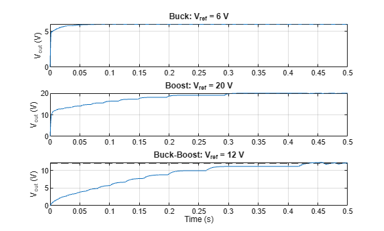
$Figure contains 3 axes objects. Axes object 1 with title Buck: V indexOf ref baseline = 6 V, ylabel V_{out} (V) contains 2 objects of type line, constantline. Axes object 2 with title Boost: V indexOf ref baseline = 20 V, ylabel V_{out} (V) contains 2 objects of type line, constantline. Axes object 3 with title Buck-Boost: V indexOf ref baseline = 12 V, xlabel Time (s), ylabel V_{out} (V) contains 2 objects of type line, constantline.$

The Buck converter settles fastest because it has no RHP zero and uses a small 10 µF output capacitor. The Boost converter settles near its reference by 0.5 s with a small overshoot despite its RHP zero, because the compensator design accounts for the bandwidth ceiling. The Buck-Boost converter exhibits a negative initial transient unique to the inverting topology and converges toward 12 V by the end of the simulation, with the final approach slowed by the 4700 µF capacitor.

To compare the normalized transient shape across topologies, plot each response as a fraction of its voltage reference. This removes the effect of different voltage levels and reveals the relative settling behavior directly.

buckNorm = buckCLVfb.Data / 6;
boostNorm = boostCLVfb.Data / 20;
bbNorm = bbCLVfb.Data / 12;

figure
plot(buckCLVfb.Time, buckNorm, ...
     boostCLVfb.Time, boostNorm, ...
     bbCLVfb.Time, bbNorm)
yline(1, "--", "V_{ref} (normalized)", LabelHorizontalAlignment="left")
xlabel("Time (s)")
ylabel("Normalized Output Voltage")
title("Normalized Closed-Loop Output Voltage Comparison")
legend("Buck", "Boost", "Buck-Boost", Location="southeast")
grid on

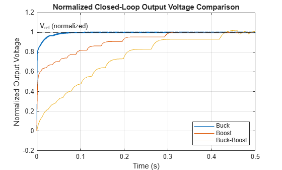
Figure contains an axes object. The axes object with title Normalized Closed-Loop Output Voltage Comparison, xlabel Time (s), ylabel Normalized Output Voltage contains 4 objects of type line, constantline. These objects represent Buck, Boost, Buck-Boost.

The normalized plot confirms that the Buck converter converges most rapidly with a small, well-damped overshoot. The Boost converter follows a similar profile over a longer time scale. The Buck-Boost converter dips below zero before rising toward the reference. This startup behavior is characteristic of the inverting topology and does not appear in the Buck or Boost designs.

Conclusion

You simulated voltage mode PI control for Buck, Boost, and Buck-Boost converters using the DCDC Controller Parameters and DCDC Voltage Controller blocks. Each topology uses a different steady-state duty cycle formula: $D = V_{o u t} / V_{i n}$ for the Buck, $D = 1 - V_{i n} / V_{o u t}$ for the Boost, and $D = V_{o u t} / (V_{i n} + V_{o u t})$ for the Buck-Boost. The LoopSelect parameter lets you switch between a fixed open-loop duty cycle and active PI regulation without modifying the model structure.

The PI gains for each closed-loop simulation come from the DCDC Controller Parameters block, which derives them from the plant dialog values when CtrlCalType is set to Compute from dialog parameters. To adapt any of these examples to a new plant, edit the corresponding *VoltageControlData.m script. The block recomputes gains automatically when the model updates. To hand-tune Kp and Ki instead, set CtrlCalType to Custom Inputs on the block dialog.