Nonlinear MPC Controller
Simulate nonlinear model predictive controllers
Libraries:
Model Predictive Control Toolbox
Description
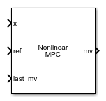
The Nonlinear MPC Controller block simulates a nonlinear model predictive controller. At each control interval, the block computes optimal control moves by solving a nonlinear programming problem. For more information on nonlinear MPC, see Nonlinear MPC.
To use this block, you must first create an nlmpc object in the
MATLAB® workspace.
Examples
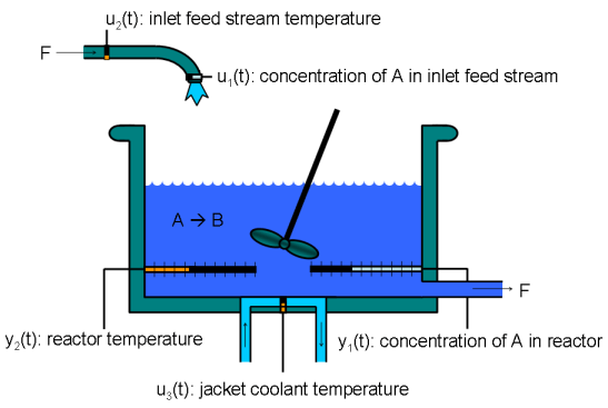
Nonlinear Model Predictive Control of Exothermic Chemical Reactor
Control a nonlinear plant as it transitions between operating points.
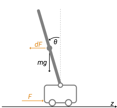
Swing-Up Control of Pendulum Using Nonlinear Model Predictive Control
Achieve swing-up and balancing control of an inverted pendulum on a cart using a nonlinear model predictive controller.

Nonlinear and Gain-Scheduled MPC Control of an Ethylene Oxidation Plant
You can generate one or more linear MPC controllers from a nonlinear MPC controller and use these controllers for gain-scheduled control applications.

Economic MPC Control of Ethylene Oxide Production
Maximize production of an ethylene oxide plant for profit using a nonlinear cost function and nonlinear constraints.
Limitations
None of the Nonlinear MPC Controller block parameters are tunable.
Ports
Input
Required Inputs
Current prediction model states, specified as a vector signal of length Nx, where Nx is the number of prediction model states. Because the nonlinear MPC controller does not perform state estimation, you must either measure or estimate the current prediction model states at each control interval.
Plant output reference values, specified as a row vector signal or matrix signal.
To use the same reference values across the prediction horizon, connect ref to a row vector signal with Ny elements, where Ny is the number of output variables. Each element specifies the reference for an output variable.
To vary the references over the prediction horizon (previewing) from time k+1 to time k+p, connect ref to a matrix signal with Ny columns and up to p rows. Here, k is the current time and p is the prediction horizon. Each row contains the references for one prediction horizon step. If you specify fewer than p rows, the final references are used for the remaining steps of the prediction horizon.
Control signals used in plant at previous control interval, specified as a vector signal of length Nmv, where Nmv is the number of manipulated variables.
Note
Connect last_mv to the MV signals actually applied to the plant in the previous control interval. Typically, these MV signals are the values generated by the controller, though this is not always the case. For example, if your controller is offline and running in tracking mode; that is, the controller output is not driving the plant, then feeding the actual control signal to last_mv can help achieve bumpless transfer when the controller is switched back online.
Additional Inputs
If your controller prediction model has measured disturbances you must enable this port and connect to it a row vector or matrix signal.
To use the same measured disturbance values across the prediction horizon, connect md to a row vector signal with Nmd elements, where Nmd is the number of manipulated variables. Each element specifies the value for a measured disturbance.
To vary the disturbances over the prediction horizon (previewing) from time k to time k+p, connect md to a matrix signal with Nmd columns and up to p+1 rows. Here, k is the current time and p is the prediction horizon. Each row contains the disturbances for one prediction horizon step. If you specify fewer than p+1 rows, the final disturbances are used for the remaining steps of the prediction horizon.
Dependencies
To enable this port, select the Measured disturbances parameter.
If your controller uses optional parameters in its prediction model, custom cost
function, or custom constraint functions, enable this input port, and connect a
parameter bus signal with Np elements, where
Np is the number of parameters. For more
information on creating a parameter bus signal, see createParameterBus. The controller passes these parameters to its model
functions, cost function, constraint functions, passivity functions and Jacobian
functions.
If your controller does not use optional parameters, you must disable params.
Dependencies
To enable this port, select the Model parameters parameter.
To specify manipulated variable targets, enable this input port, and connect a vector signal. To make a given manipulated variable track its specified target value, you must also specify a nonzero tuning weight for that manipulated variable.
The supplied mv.target values at run-time apply across the prediction horizon.
Dependencies
To enable this port, select the Targets for manipulated variables parameter.
Online Constraints
To specify run-time minimum output variable constraints, enable this input port.
If this port is disabled, the block uses the lower bounds specified in the
OutputVariables.Min property of its controller object.
To use the same bounds over the prediction horizon, connect y.min to a row vector signal with Ny elements, where Ny is the number of outputs. Each element specifies the lower bound for an output variable.
To vary the bounds over the prediction horizon from time k+1 to time k+p, connect y.min to a matrix signal with Ny columns and up to p rows. Here, k is the current time and p is the prediction horizon. Each row contains the bounds for one prediction horizon step. If you specify fewer than p rows, the bounds in the final row apply for the remainder of the prediction horizon.
Dependencies
To enable this port, select the Lower OV limits parameter.
To specify run-time maximum output variable constraints, enable this input port.
If this port is disabled, the block uses the upper bounds specified in the
OutputVariables.Min property of its controller object.
To use the same bounds over the prediction horizon, connect y.max to a row vector signal with Ny elements, where Ny is the number of outputs. Each element specifies the upper bound for an output variable.
To vary the bounds over the prediction horizon from time k+1 to time k+p, connect y.max to a matrix signal with Ny columns and up to p rows. Here, k is the current time and p is the prediction horizon. Each row contains the bounds for one prediction horizon step. If you specify fewer than p rows, the bounds in the final row apply for the remainder of the prediction horizon.
Dependencies
To enable this port, select the Upper OV limits parameter.
To specify run-time minimum manipulated variable constraints, enable this input port.
If this port is disabled, the block uses the lower bounds specified in the
ManipulatedVariables.Min property of its controller
object.
To use the same bounds over the prediction horizon, connect mv.min to a row vector signal with Nmv elements, where Nmv is the number of outputs. Each element specifies the lower bound for a manipulated variable.
To vary the bounds over the prediction horizon from time k to time k+p–1, connect mv.min to a matrix signal with Ny columns and up to p rows. Here, k is the current time and p is the prediction horizon. Each row contains the bounds for one prediction horizon step. If you specify fewer than p rows, the bounds in the final row apply for the remainder of the prediction horizon.
Dependencies
To enable this port, select the Lower MV limits parameter.
To specify run-time maximum manipulated variable constraints, enable this input port.
If this port is disabled, the block uses the upper bounds specified in the
ManipulatedVariables.Max property of its controller
object.
To use the same bounds over the prediction horizon, connect mv.max to a row vector signal with Nmv elements, where Nmv is the number of outputs. Each element specifies the upper bound for a manipulated variable.
To vary the bounds over the prediction horizon from time k to time k+p–1, connect mv.max to a matrix signal with Ny columns and up to p rows. Here, k is the current time and p is the prediction horizon. Each row contains the bounds for one prediction horizon step. If you specify fewer than p rows, the bounds in the final row apply for the remainder of the prediction horizon.
Dependencies
To enable this port, select the Upper MV limits parameter.
To specify run-time minimum manipulated variable rate constraints, enable this
input port. If this port is disabled, the block uses the lower bounds specified in the
ManipulatedVariable.RateMin property of its controller object.
dmv.min bounds must be nonpositive.
To use the same bounds over the prediction horizon, connect dmv.min to a row vector signal with Nmv elements, where Nmv is the number of outputs. Each element specifies the lower bound for a manipulated variable rate of change.
To vary the bounds over the prediction horizon from time k to time k+p–1, connect dmv.min to a matrix signal with Ny columns and up to p rows. Here, k is the current time and p is the prediction horizon. Each row contains the bounds for one prediction horizon step. If you specify fewer than p rows, the bounds in the final row apply for the remainder of the prediction horizon.
Dependencies
To enable this port, select the Lower MVRate limits parameter.
To specify run-time maximum manipulated variable rate constraints, enable this input
port. If this port is disabled, the block uses the upper bounds specified in the
ManipulatedVariables.RateMax property of its controller object.
dmv.max bounds must be nonnegative.
To use the same bounds over the prediction horizon, connect dmv.max to a row vector signal with Nmv elements, where Nmv is the number of outputs. Each element specifies the upper bound for a manipulated variable rate of change.
To vary the bounds over the prediction horizon from time k to time k+p–1, connect dmv.max to a matrix signal with Ny columns and up to p rows. Here, k is the current time and p is the prediction horizon. Each row contains the bounds for one prediction horizon step. If you specify fewer than p rows, the bounds in the final row apply for the remainder of the prediction horizon.
Dependencies
To enable this port, select the Upper MVRate limits parameter.
To specify run-time minimum state constraints, enable this input port. If this port is
disabled, the block uses the lower bounds specified in the States.Min
property of its controller object.
To use the same bounds over the prediction horizon, connect x.min to a row vector signal with Nx elements, where Nx is the number of outputs. Each element specifies the lower bound for a state.
To vary the bounds over the prediction horizon from time k+1 to time k+p, connect x.min to a matrix signal with Ny columns and up to p rows. Here, k is the current time and p is the prediction horizon. Each row contains the bounds for one prediction horizon step. If you specify fewer than p rows, the bounds in the final row apply for the remainder of the prediction horizon.
Dependencies
To enable this port, select the Lower state limits parameter.
To specify run-time maximum state constraints, enable this input port. If this port is
disabled, the block uses the upper bounds specified in the States.Max
property of its controller object.
To use the same bounds over the prediction horizon, connect x.max to a row vector signal with Nx elements, where Nx is the number of outputs. Each element specifies the upper bound for a state.
To vary the bounds over the prediction horizon from time k+1 to time k+p, connect x.max to a matrix signal with Ny columns and up to p rows. Here, k is the current time and p is the prediction horizon. Each row contains the bounds for one prediction horizon step. If you specify fewer than p rows, the bounds in the final row apply for the remainder of the prediction horizon.
Dependencies
To enable this port, select the Upper state limits parameter.
Online Tuning Weights
To specify run-time output variable tuning weights, enable this input port. If this port is disabled, the block uses the tuning weights specified in the Weights.OutputVariables property of its controller object. These tuning weights penalize deviations from output references.
If the MPC controller object uses constant output tuning weights over the prediction horizon, you can specify only constant output tuning weights at runtime. Similarly, if the MPC controller object uses output tuning weights that vary over the prediction horizon, you can specify only time-varying output tuning weights at runtime.
To use constant tuning weights over the prediction horizon, connect y.wt to a row vector signal with Ny elements, where Ny is the number of outputs. Each element specifies a nonnegative tuning weight for an output variable. For more information on specifying tuning weights, see Tune Weights.
To vary the tuning weights over the prediction horizon from time k+1 to time k+p, connect y.wt to a matrix signal with Ny columns and up to p rows. Here, k is the current time and p is the prediction horizon. Each row contains the tuning weights for one prediction horizon step. If you specify fewer than p rows, the tuning weights in the final row apply for the remainder of the prediction horizon. For more information on varying weights over the prediction horizon, see Setting Time-Varying Weights and Constraints with MPC Designer.
Dependencies
To enable this port, select the OV weights parameter.
To specify run-time manipulated variable tuning weights, enable this input port.
If this port is disabled, the block uses the tuning weights specified in the
Weights.ManipulatedVariables property of its controller object.
These tuning weights penalize deviations from MV targets.
To use the same tuning weights over the prediction horizon, connect mv.wt to a row vector signal with Nmv elements, where Nmv is the number of manipulated variables. Each element specifies a nonnegative tuning weight for a manipulated variable. For more information on specifying tuning weights, see Tune Weights.
To vary the tuning weights over the prediction horizon from time k to time k+p-1, connect mv.wt to a matrix signal with Nmv columns and up to p rows. Here, k is the current time and p is the prediction horizon. Each row contains the tuning weights for one prediction horizon step. If you specify fewer than p rows, the tuning weights in the final row apply for the remainder of the prediction horizon. For more information on varying weights over the prediction horizon, see Setting Time-Varying Weights and Constraints with MPC Designer.
Dependencies
To enable this port, select the MV weights parameter.
To specify run-time manipulated variable rate tuning weights, enable this input
port. If this port is disabled, the block uses the tuning weights specified in the
Weights.ManipulatedVariablesRate property of its controller
object. These tuning weights penalize large changes in control moves.
To use the same tuning weights over the prediction horizon, connect dmv.wt to a row vector signal with Nmv elements, where Nmv is the number of manipulated variables. Each element specifies a nonnegative tuning weight for a manipulated variable rate. For more information on specifying tuning weights, see Tune Weights.
To vary the tuning weights over the prediction horizon from time k to time k+p-1, connect dmv.wt to a matrix signal with Nmv columns and up to p rows. Here, k is the current time and p is the prediction horizon. Each row contains the tuning weights for one prediction horizon step. If you specify fewer than p rows, the tuning weights in the final row apply for the remainder of the prediction horizon. For more information on varying weights over the prediction horizon, see Setting Time-Varying Weights and Constraints with MPC Designer.
Dependencies
To enable this port, select the MVRate weights parameter.
To specify a run-time slack variable tuning weight, enable this input port and connect a scalar signal. If this port is disabled, the block uses the tuning weight specified in the Weights.ECR property of its controller object.
The slack variable tuning weight has no effect unless your controller object defines soft constraints whose associated ECR values are nonzero. If there are soft constraints, increasing the ecr.wt value makes these constraints relatively harder. The controller then places a higher priority on minimizing the magnitude of the predicted worst-case constraint violation.
Dependencies
To enable this port, select the ECR weight parameter.
Initial Guesses
To specify initial guesses for the optimal manipulated variable solutions, enable this input port. If this port is disabled, the block uses the optimal control sequences calculated in the previous control interval as initial guesses.
To use the same initial guesses over the prediction horizon, connect mv.init to a vector signal with Nmv elements, where Nmv is the number of manipulated variables. Each element specifies the initial guess for a manipulated variable.
To vary the initial guesses over the prediction horizon from time k to time k+p-1, connect mv.init to a matrix signal with Nmv columns and up to p rows. Here, k is the current time and p is the prediction horizon. Each row contains the initial guesses for one prediction horizon step. If you specify fewer than p rows, the guesses in the final row apply for the remainder of the prediction horizon.
Dependencies
To enable this port, select the Initial guess parameter.
To specify initial guesses for the optimal state solutions, enable this input port. If this port is disabled, the block uses the optimal state sequences calculated in the previous control interval as initial guesses.
To use the same initial guesses over the prediction horizon, connect x.init to a vector signal with Nx elements, where Nx is the number of states. Each element specifies the initial guess for a state.
To vary the initial guesses over the prediction horizon from time k to time k+p-1, connect x.init to a matrix signal with Nx columns and up to p rows. Here, k is the current time and p is the prediction horizon. Each row contains the initial guesses for one prediction horizon step. If you specify fewer than p rows, the guesses in the final row apply for the remainder of the prediction horizon.
Dependencies
To enable this port, select the Initial guess parameter.
To specify an initial guess for the slack variable used for constraint softening
at the solution, enable this input port and connect a nonnegative scalar signal. If
this port is disabled, the block uses an initial guess of 0.
Dependencies
To enable this port, select the Initial guess parameter.
Output
Required Output
Optimal manipulated variable control action, output as a column vector signal of length Nmv, where Nmv is the number of manipulated variables.
If the solver converges to a local optimum solution (nlp.status is positive), then mv contains the optimal solution.
If the solver reaches the maximum number of iterations without finding an optimal
solution (nlp.status is zero) and the
Optimization.UseSuboptimalSolution property of the controller
is:
true, then mv contains the suboptimal solution.false, then mv is the same as last_mv.
If the solver fails (nlp.status is negative), then mv is the same as last_mv.
Additional Outputs
Objective function cost, output as a nonnegative scalar signal. The cost quantifies the degree to which the controller has achieved its objectives.
The cost value is meaningful only when the nlp.status output is nonnegative.
Dependencies
To enable this port, select the Optimal cost parameter.
Slack variable, ε, used in constraint softening, output as 0 or
a positive scalar value.
ε = 0 — All soft constraints are satisfied over the entire prediction horizon.
ε > 0 — At least one soft constraint is violated. When more than one constraint is violated, ε represents the worst-case soft constraint violation (scaled by the ECR values for each constraint).
Dependencies
To enable this port, select the Slack variable parameter.
Optimization status, output as one of the following:
Positive Integer — Solver converged to an optimal solution
0— Maximum number of iterations reached without converging to an optimal solutionNegative integer — Solver failed
Dependencies
To enable this port, select the Optimization status parameter.
Optimal Sequences
Optimal manipulated variable sequence, returned as a matrix signal with p+1 rows and Nmv columns, where p is the prediction horizon and Nmv is the number of manipulated variables.
The first p rows of mv.seq contain the calculated optimal manipulated variable values from current time k to time k+p-1. The first row of mv.seq contains the current manipulated variable values (output mv). Because the controller does not calculate optimal control moves at time k+p, the final two rows of mv.seq are identical.
Dependencies
To enable this port, select the Optimal control sequence parameter.
Optimal prediction model state sequence, returned as a matrix signal with p+1 rows and Nx columns, where p is the prediction horizon and Nx is the number of states.
The first row of x.seq contains the current estimated state values, either from the built-in state estimator or from the custom state estimation block input x[k|k]. The next p rows of x.seq contain the calculated optimal state values from time k+1 to time k+p.
Dependencies
To enable this port, select the Optimal state sequence parameter.
Optimal output variable sequence, returned as a matrix signal with p+1 rows and Ny columns, where p is the prediction horizon and Ny is the number of output variables.
The first p rows of y.seq contain the calculated optimal output values from current time k to time k+p-1. The first row of y.seq is computed based on the current estimated states and the current measured disturbances (first row of input md). Because the controller does not calculate optimal output values at time k+p, the final two rows of y.seq are identical.
Dependencies
To enable this port, select the Optimal output sequence parameter.
Parameters
You must provide an nlmpc object
that defines a nonlinear MPC controller. To do so, enter the name of an
nlmpc object in the MATLAB workspace.
Programmatic Use
Block Parameter:
nlmpcobj |
| Type: string, character vector |
Default:
"" |
General Tab
If your controller has measured disturbances, you must select this parameter to add the md output port to the block.
Programmatic Use
Block Parameter:
md_enabled |
| Type: string, character vector |
Values:
"off", "on" |
Default:
"off" |
Select this parameter to add the mv.target input port to the block.
Programmatic Use
Block Parameter:
mvtarget_enabled |
| Type: string, character vector |
Values:
"off", "on" |
Default:
"off" |
If your controller uses optional parameters, you must select this parameter to add the params output port to the block.
For more information on creating a parameter bus signal, see createParameterBus.
Programmatic Use
Block Parameter:
param_enabled |
| Type: string, character vector |
Values:
"off", "on" |
Default:
"off" |
Select this parameter to add the cost output port to the block.
Programmatic Use
Block Parameter:
cost_enabled |
| Type: string, character vector |
Values:
"off", "on" |
Default:
"off" |
Select this parameter to add the mv.seq output port to the block.
Programmatic Use
Block Parameter:
mvseq_enabled |
| Type: string, character vector |
Values:
"off", "on" |
Default:
"off" |
Select this parameter to add the x.seq output port to the block.
Programmatic Use
Block Parameter:
stateseq_enabled |
| Type: string, character vector |
Values:
"off", "on" |
Default:
"off" |
Select this parameter to add the y.seq output port to the block.
Programmatic Use
Block Parameter:
ovseq_enabled |
| Type: string, character vector |
Values:
"off", "on" |
Default:
"off" |
Select this parameter to add the slack output port to the block.
Programmatic Use
Block Parameter:
slack_enabled |
| Type: string, character vector |
Values:
"off", "on" |
Default:
"off" |
Select this parameter to add the nlp.status output port to the block.
Programmatic Use
Block Parameter:
status_enabled |
| Type: string, character vector |
Values:
"off", "on" |
Default:
"off" |
Online Features Tab
Select this parameter to add the ov.min input port to the block.
Programmatic Use
Block Parameter:
ov_min |
| Type: string, character vector |
Values:
"off", "on" |
Default:
"off" |
Select this parameter to add the ov.max input port to the block.
Programmatic Use
Block Parameter:
ov_max |
| Type: string, character vector |
Values:
"off", "on" |
Default:
"off" |
Select this parameter to add the mv.min input port to the block.
Programmatic Use
Block Parameter:
mv_min |
| Type: string, character vector |
Values:
"off", "on" |
Default:
"off" |
Select this parameter to add the mv.max input port to the block.
Programmatic Use
Block Parameter:
mv_max |
| Type: string, character vector |
Values:
"off", "on" |
Default:
"off" |
Select this parameter to add the dmv.min input port to the block.
Programmatic Use
Block Parameter: mvrate_min |
| Type: string, character vector |
Values: "off", "on" |
Default: "off" |
Select this parameter to add the dmv.max input port to the block.
Programmatic Use
Block Parameter: mvrate_max |
| Type: string, character vector |
Values: "off", "on" |
Default: "off" |
Select this parameter to add the x.min input port to the block.
Programmatic Use
Block Parameter: state_min |
| Type: string, character vector |
Values: "off", "on" |
Default: "off" |
Select this parameter to add the x.max input port to the block.
Programmatic Use
Block Parameter: state_max |
| Type: string, character vector |
Values: "off", "on" |
Default: "off" |
Select this parameter to add the y.wt input port to the block.
Programmatic Use
Block Parameter:
ov_weight |
| Type: string, character vector |
Values:
"off", "on" |
Default:
"off" |
Select this parameter to add the mv.wt input port to the block.
Programmatic Use
Block Parameter:
mv_weight |
| Type: string, character vector |
Values:
"off", "on" |
Default:
"off" |
Select this parameter to add the dmv.wt input port to the block.
Programmatic Use
Block Parameter:
mvrate_weight |
| Type: string, character vector |
Values:
"off", "on" |
Default:
"off" |
Select this parameter to add the ecr.wt input port to the block.
Programmatic Use
Block Parameter:
ecr_weight |
| Type: string, character vector |
Values:
"off", "on" |
Default:
"off" |
Select this parameter to add the mv.init, x.init, and e.init input ports to the block.
Note
By default, the Nonlinar MPC Controller block uses the calculated optimal manipulated variable and state trajectories from one control interval as the initial guesses for the next control interval.
Enable the initial guess ports only if it is necessary for your application.
Programmatic Use
Block Parameter:
nlp_initialize |
| Type: string, character vector |
Values:
"off", "on" |
Default:
"off" |
Others Tab
Specify the data type of the manipulated variables, and the floating point precision that the block uses to compute them, as one of the following:
double— The block uses double-precision floating point to store arrays and compute the manipulated variables.single— The block uses single-precision floating point to store arrays and compute the manipulated variables.If you are implementing the block on a single-precision target, specify the output data type as
single.<data type expression>— An expression that evaluates to eitherdoubleorsingle. For more information see Control Data Types of Signals (Simulink).
Programmatic Use
Block Parameter: BlockDataType |
| Type: string, character vector |
Values:
"double", "single", data type
expression |
Default: "double" |
Select this parameter to run the controller using the same sample time as its prediction model. To use a different controller sample time, clear this parameter, and specify the sample time using the Make block run at a different sample time parameter.
To limit the number of decision variables and improve computational efficiency, you can run the controller with a sample time that is different from the prediction horizon. For example, consider the case of a nonlinear MPC controller running at 10 Hz. If the plant and controller sample times match, predicting plant behavior for ten seconds requires a prediction horizon of length 100, which produces a large number of decision variables. To reduce the number of decision variables, you can use a plant sample time of 1 second and a prediction horizon of length 10.
Programmatic Use
Block Parameter:
UseObjectTs |
| Type: string, character vector |
Values:
"off", "on" |
Default:
"on" |
Specify this parameter to run the controller using a different sample time from its
prediction model. Setting this parameter to -1 allows the block to
inherit the sample time from its parent subsystem.
Note
The first element of the MV rate vector (which is the difference between the current and the last value of the manipulated variable) is normally weighted and constrained assuming that the last value of the MV occurred in the past at the sample time specified in the MPC object. When the block is executed with a different sample rate, this assumption no longer holds, therefore, in this case, you must make sure that the weights and constraints defined in the controller handle the first element of the MV rate vector correctly.
Dependencies
To enable this parameter, clear the Use prediction model sample time parameter.
Programmatic Use
Block Parameter:
TsControl |
| Type: string, character vector |
Default:
"" |
Select this parameter to simulate the controller using a MEX function generated using
buildMEX. Doing so reduces the simulation time of the
controller. To specify the name of the MEX function, use the Specify MEX
function name parameter.
Programmatic Use
Block Parameter:
UseMEX |
| Type: string, character vector |
Values:
"off", "on" |
Default:
"off" |
Use this parameter to specify the name of the MEX function to use during simulation.
To create the MEX function, use the buildMEX function.
Dependencies
To enable this parameter, select the Use MEX to speed up simulation parameter.
Programmatic Use
Block Parameter:
mexname |
| Type: string, character vector |
Default:
"" |
Extended Capabilities
Usage notes and limitations:
The Nonlinear MPC Controller block supports generating code only for nonlinear MPC controllers that use the default
fminconsolver with the SQP algorithm.Code generation for single-precision or fixed-point computations is not supported.
When used for code generation, nonlinear MPC controllers do not support expressing prediction model functions, stage cost functions or constraint functions as anonymous functions.
If your controller uses optional parameters, you must also generate code for the Bus Creator block connected to the params input port. To do so, place the Nonlinear MPC Controller and Bus Creator blocks within a subsystem, and generate code for that subsystem.
The Support non-finite numbers check box in the Interface section of the Code Generation options, under the model Configuration Parameters dialog box, must be checked (default option).
When generating code using Embedded Coder®, the Support variable-size signals in the Interface section of the Code Generation options, under the model Configuration Parameters dialog box, must be checked. By default this check box is unchecked and you must check it before generating code.
Version History
Introduced in R2018b
See Also
Blocks
Functions
Objects
Topics
MATLAB Command
You clicked a link that corresponds to this MATLAB command:
Run the command by entering it in the MATLAB Command Window. Web browsers do not support MATLAB commands.
Seleziona un sito web
Seleziona un sito web per visualizzare contenuto tradotto dove disponibile e vedere eventi e offerte locali. In base alla tua area geografica, ti consigliamo di selezionare: .
Puoi anche selezionare un sito web dal seguente elenco:
Come ottenere le migliori prestazioni del sito
Per ottenere le migliori prestazioni del sito, seleziona il sito cinese (in cinese o in inglese). I siti MathWorks per gli altri paesi non sono ottimizzati per essere visitati dalla tua area geografica.
Americhe
- América Latina (Español)
- Canada (English)
- United States (English)
Europa
- Belgium (English)
- Denmark (English)
- Deutschland (Deutsch)
- España (Español)
- Finland (English)
- France (Français)
- Ireland (English)
- Italia (Italiano)
- Luxembourg (English)
- Netherlands (English)
- Norway (English)
- Österreich (Deutsch)
- Portugal (English)
- Sweden (English)
- Switzerland
- United Kingdom (English)