Avoid Obstacles Using TEB Local Planner in Simulink
This example shows how to use the Timed Elastic Band block in Simulink® for local path planning to avoid obstacles. The block implements the Timed Elastic Band (TEB) algorithm to compute optimal path while considering vehicle kinematic constraints. The SolnInfo output of the block specifies whether an optimal path is feasible. The LastFeasibleIdx and ExitFlag fields in the SolnInfo output bus indicate whether an optimal path is feasible at a given timestamp. The LastFeasibleIdx specifies a pose along the optimal path and denotes the timestamp up to which the trajectory is feasible. For each timestamp after the one specified by LastFeasibleIdx, the value of ExitFlag is greater than zero and indicates an error in computing the optimal path. This example shows how to address these errors and generate an optimal path to maneuver the vehicle from the start pose to the goal pose.
An
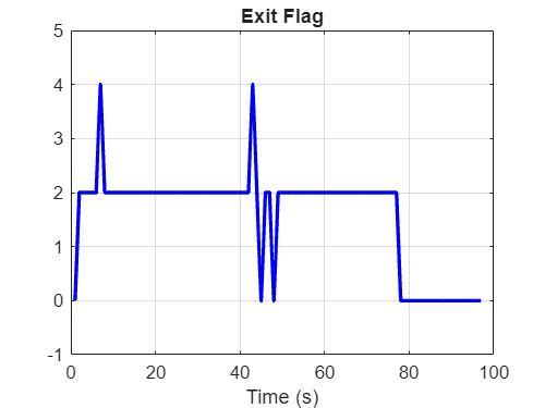
ExitFlagvalue of1indicates a collision with an obstacle on the trajectory afterLastFeasibleIdxlie on the obstacles. The model sets theLastfeasibleIdxas the current pose and continues to optimize the local path.ExitFlagvalue of2indicates that the vehicle does not maintain a safe distance from obstacles at the corresponding timestamp, violating the obstacle safety margin constraint by more than 10%.ExitFlagvalue of3indicates that the turning radius of the vehicle while moving from the current pose to a subsequent pose violates the minimum turning radius constraint by more than 10%.ExitFlagvalue of4indicates that the timestamp of the planner has not updated correctly.If the value of
LastFeasibleIdxvalue is1, the path becomes infeasible immediately after the first state. This indicates that the planner could not find a valid path beyond the current pose.
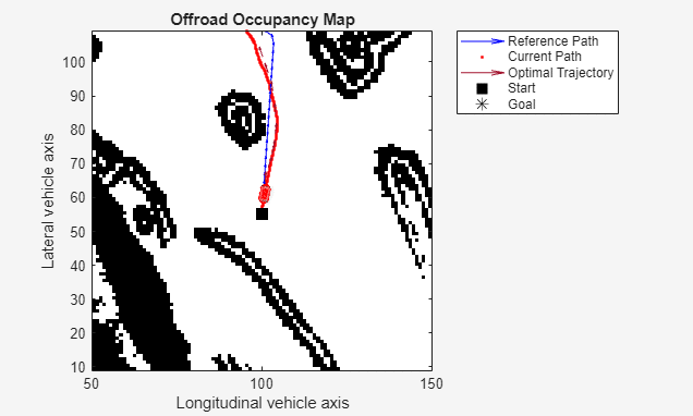
The simulation highlights path following and obstacle avoidance, where the robot adheres to the planned trajectory as it navigates through the environment.
Overview of Model
Open the Simulink model.
open_system("PathFollowingTEB.slx")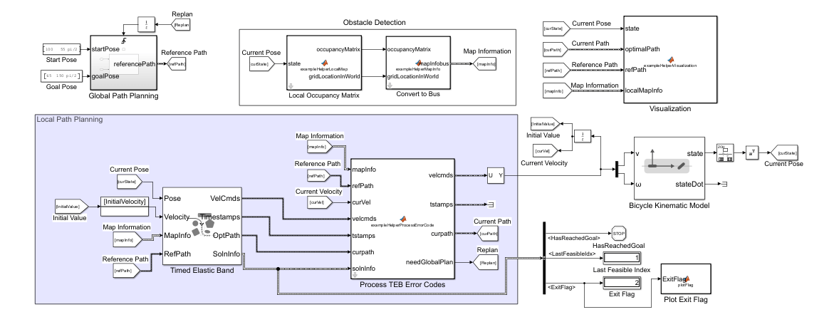
The Simulink model for local path planning using the TEB algorithm primarily consists of four main components: Global Path Planning, Obstacle Detection, Local Path Planning, and Visualization.
The model also uses a Bicycle Kinematic Model block to compute the current pose for the vehicle by using the velocity commands computed during local planning. The Bicycle Kinematic Model block considers the kinematic constraints of the vehicle while computing the current pose.
The Timed Elastic Band block returns the SolnInfo output as a bus.
The
ExitFlagand theLastFeasibleIndexblocks display the values of theExitFlagandLastFeasibleIdxfields in the SolnInfo bus, respectively, as computed by the Timed Elastic Band block at each timestamp.
The rest of the example explains each component of the model, outlines the steps involved in local path planning and error correction to generate an optimal path between the start pose and the goal pose.
Global Path Planning
The Global Path Planning component computes a reference path for the vehicle to navigate from a start pose to a goal pose on a specified map environment. The component uses the Global Path Planning MATLAB® Function block to execute the path planning strategy. Use the Global Path Planning MATLAB Function block to compute the reference path by following these steps:
Load a map that represents the environment for the vehicle. To load a custom map environment, edit the
GlobalPathPlanningMATLAB Function block and specify the name of the MAT file containing the desired map.
function referencePath = exampleHelperGlobalPlanner(startPose,goalPose)
persistent refPath mapMatrix resolution

if isempty(refPath)
    % Load Map Matrix
    data = load("offroadMap.mat","map");
    mapMatrix = data.map;
    resolution = 1;
end
Create a 2-D occupancy map for the provided environment.
Create a Dubins state space object, and set the minimum turning radius for the vehicle. In this example, the minimum turning radius is set to 2 m.
Create a state validator object to check the validity of states.
Configure the RRT* path planner, and plan a path from the start pose to the goal pose using the RRT* path planner.
Optimize the computed path by removing unnecessary waypoints.
The Global Path Planning components contains a trigger that replans the reference path if the vehicle is unable to follow the reference path to navigate from the start pose to the goal pose. This triggers if the current pose estimated by the TEB local path planner is the same as the previous pose.
Obstacle Detection
The Obstacle Detection component generates a local occupancy matrix that indicates which areas around the vehicle are occupied or free.
The
ObstacleDetectioncomponent uses theLocalOccupancyMatrixMATLAB Function block to generate an egocentric local map. The map is centered on the vehicle and extends to cover a defined area that include the immediate field of view of the vehicle. In this example, the area is determined as twice the maximum distance the vehicle can travel in a single iteration and the maximum distance is set to 50 m. TheLocalOccupancyMatrixMATLAB Function block continuously updates the local map to reflect the current pose of the vehicle. This involves moving the map to align with the current pose of the vehicle and synchronizing it with the global map to ensure consistency. The Bicycle Kinematics Model block provides the current pose of the vehicle at each time step. The global map provides a comprehensive view of the entire area, and the local map focuses on the immediate surroundings of the vehicle and, updating in real-time to reflect dynamic changes.The
LocalOccupancyMatrixMATLAB Function block outputs the occupancy matrix from the local map and provides the grid location in the world coordinate system.
function [occupancyMatrix,gridLocationInWorld] = exampleHelperLocalMap(state)
% The exampleHelperLocalMap block generates an occupancy matrix to detect ...
% obstacles within the field of view. % It simulates sensors like lidar or ...
% cameras to produce occupancy data in a matrix format for further processing.

persistent globalMap localMap

if isempty(globalMap)
 % Load an occupancy map.
 data = load("offroadMap.mat","map");
 globalMap =   binaryOccupancyMap(data.map);
The
ObstacleDetectioncomponent stores the map information from theLocalOccupancyMatrixMATLAB Function block as a bus signal. The component uses theConverttoBusMATLAB Function block to store the occupancy matrix and grid information in a bus signal. Use the block parameters to specify the grid size, the map resolution, and the grid origin in local coordinates.
function mapInfobus = exampleHelperMapInfo(occupancyMatrix,gridLocationInWorld,GridSize,Resolution,GridOriginInLocal)
persistent mapInfoStruct
if isempty(mapInfoStruct)

    % Create occupancy matrix from grid size.
    occupancyMatrix = false(GridSize);

    % Create struct to contain essential information to create map
    mapInfoStruct = struct('Resolution',Resolution,'GridLocationInWorld', ...
        gridLocationInWorld,'OccupancyMatrix' occupancyMatrix,'GridSize', ...
        GridSize,'GridOriginInLocal', GridOriginInLocal);
end

mapInfoStruct.GridLocationInWorld = gridLocationInWorld; % Update map location in world.
mapInfoStruct.OccupancyMatrix = occupancyMatrix; % Update occupancy map
mapInfobus = mapInfoStruct;
end
Local Path Planning
The Local Path Planning component uses the Timed Elastic Band block to compute the velocity commands that direct the vehicle to follow the specified reference path while avoiding obstacles. The Timed Elastic Band block:
Uses the map information from the
ObstacleDetectioncomponent to detect and avoid obstacles.Modifies the trajectory of the vehicle to maintain proximity to the reference path while avoiding obstacles. The block obtains the reference path from the
GlobalPathPlanningcomponent.Considers the kinematic constraints of the vehicle, such as maximum velocity, minimum turning radius, and acceleration limits, to ensure feasible motion. Use the Timed Elastic Band block parameters to specify the trajectory parameters. For details on these parameters and how to set their values, see the Parameters section of the Timed Elastic Band block.
The Timed Elastic Band block returns these values:
Velocity commands at each timestamp, VelCmds, that include both the linear velocity and the angular velocity.
Timestamps corresponding to velocity commands.
Optimized path, OptPath, that specifies the xy-position and orientation angle (theta) of waypoints along the path at each timestamp.
Extra information, SolnInfo, that provides information about the solution derived using the Timed Elastic Band block. The
LastFeasibleIdxandExitFlagfields in the SolnInfo output bus indicate the status of the local path planning.
Error Correction
The Local Path Planning component uses the Process TEB Error Codes MATLAB Function block and the exampleHelperProcessTEBErrorFlags helper function to correct errors and guide the vehicle toward the goal pose.
Obstacle Safety Margin Violated by More Than 10% (************ExitFlag = 2)
If the path generated by the TEB algorithm causes the vehicle to navigate too close to an obstacle, exceeding the safety margin constraint, the ExitFlag value for the corresponding timestamp is 2. If the specified obstacle safety margin is not significantly greater than the actual dimensions of the vehicle, violating this margin implies a potential collision. Given that the obstacle safety margin defines an additional buffer around the vehicle, you must determine whether a violation of this margin actually indicates a collision. If the violation affects only the buffer region and does not impact the vehicle itself, it implies that the vehicle can navigate without collision.
Use the exampleHelperProcessTEBErrorFlags helper function to check if the vehicle is too close to the obstacle and may cause a collision, and take appropriate action to avoid collision. Follow these steps to correct the error and generate the optimized path.
Define a minimum threshold for feasible drive duration by using the lookahead time.
Create a collision-checking configuration by considering the dimensions of the vehicle. The
exampleHelperProcessTEBErrorFlagshelper function uses theinflationCollisionCheckerfunction to determine the collision-checking configuration. TheexampleHelperVehicleSpecshelper functions specifies the dimensions of the vehicle for collision checking.Generate a signed distance map from the occupancy matrix computed by the
ObstacleDetectioncomponent.Select 2-D reference points along the length of the vehicle to use as the maximum boundary for collision checking.
Use the signed distance map to calculate the distance from each reference point on the vehicle to the nearest obstacle. Compute the minimum distance across all reference points for each pose along the path. If the distance is greater than zero or
NaN, the corresponding pose is collision-free. The positive distance indicates a safe buffer from obstacles, andNaNrepresents undefined areas where no collision is detected.Find the poses for which the computed distance is less than or equal to zero. You can consider these poses as collision points. Find the index of the first collision point and check its timestamp.
If the timestamp of the first collision point is less than the minimum threshold for feasible drive duration, the collision occurs too early in the path for local correction and the function triggers global path replanning.
If the timestamp of the first collision point is greater than the minimum threshold for feasible drive duration, trim the path and associated commands up to the last feasible index and initiate local path planning using the last feasible index as the current pose.
Minimum Turning Radius Violated by More Than 10% (************ExitFlag = 3)
If the path generated by the TEB algorithm results in a turning radius for the vehicle that is smaller than the minimum turning radius, the ExitFlag value for the corresponding timestamp is 3. This implies that the vehicle is attempting to make a turn that is tighter than allowed by the minimum turning radius constraint, exceeding this constraint by more than 10%. The discrepancy often arises from a misalignment between the actual heading angle of the vehicle and the trajectory generated by the TEB algorithm. In an effort to rectify this misalignment and adhere closely to the planned trajectory, the algorithm may inadvertently generate velocity commands that exceed the vehicle's kinematic constraints.
Use the exampleHelperProcessTEBErrorFlags helper function to adjust the linear velocity and the angular velocity of the vehicle in such a way that the radius of curvature satisfies the minimum turning radius constraint. Perform these steps to correct the error and generate the optimized path.
To adjust the linear velocity:
Define the maximum reverse velocity as the minimum permissible velocity limit and the maximum linear velocity as the maximum permissible velocity limit for the vehicle. You must configure the maximum velocity values as parameters of the Timed Elastic Band block.
Review velocity commands at each time step to identify any that exceed the defined speed limits.
Adjust out-of-range velocity commands to fit within the permissible limits.
To adjust the angular velocity,
Calculate the minimum turning radius as a ratio of the maximum linear velocity of the vehicle to its maximum angular velocity.
Calculate the radius of curvature for each set of velocity commands by taking the absolute value of the linear velocity divided by the angular velocity.
For a given velocity command, if the radius of curvature is smaller than the minimum turning radius, adjust the angular velocity by setting it to the linear velocity divided by the minimum turning radius.
Path Planning Fails Due to Unreachable Points or Local Minima (****************LastFeasibleIdx == 1)
A LastFeasibleIdx is 1, indicates that the controller has not generated a path or that nearby reference path points are unreachable. To mitigate this error, use the Process TEB Error Codes MATLAB Function block to trigger global replanning.
Bicycle Kinematic Model
The Bicycle Kinematic Model block creates a vehicle model to simulate simplified vehicle kinematics. It takes linear and angular velocities as command inputs from the Timed Elastic Band block and outputs the current position and velocity states of the vehicle. It then provides these current velocity and position states as inputs to the Timed Elastic Band block and the Obstacle Detection component to compute the next pose along the optimal path.
The model continues to perform local path planning and error correction until the vehicle reaches the goal pose.
Visualization
The Visualization MATLAB Function block plots the local path planning results and the exit flag value at each timestamp. The block uses the exampleHelperPlotMap, exampleHelperPlotVehicle, and exampleHelperBuildVehicleGraphic helper functions to plot the results. The Plot Exit Flag MATLAB Function block plots the ExitFlag values obtained at each timestamp.
Run Simulation
Set the stop time for the simulation to 100 seconds. Run the simulation to visualize the path following results. By examining the ExitFlag, you can determine how often the local path planner detected infeasible paths and the model took corrective actions to compute a feasible path for the robot to navigate to the goal pose.
sim("PathFollowingTEB.slx");
The following animation shows the result of planning in real-time.
See Also
Blocks
- Timed Elastic Band | Bicycle Kinematic Model (Robotics System Toolbox)
Functions
inflationCollisionChecker(Automated Driving Toolbox) |plannerRRTStar|controllerTEB