Design Optimization for Reaching Target Temperature
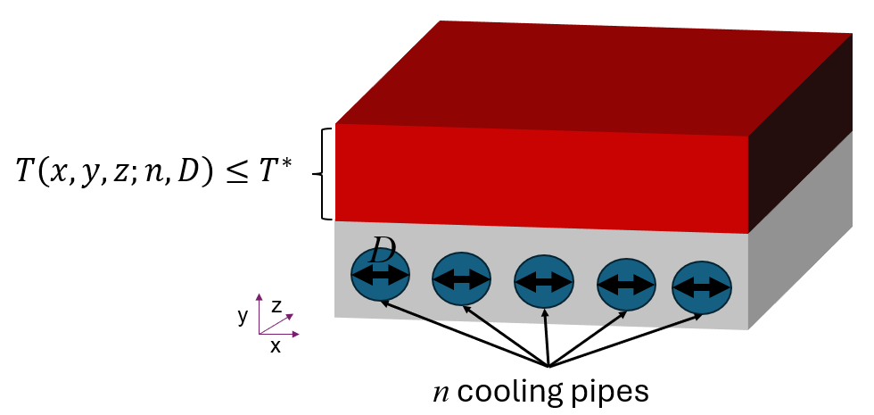
This example shows how to explore the cooling of a block via cooling pipes carrying water at a given mass flow rate. The top block is heated by a constant heat source. Optimize the number and diameter of the pipes to reach, but not exceed, a target temperature in the block.
Compute the maximum temperature in the top block by using a finite element simulation with Partial Differential Equation Toolbox™. Conduct optimization using surrogate optimization from Global Optimization Toolbox.
Geometry
For this example, you must know the region IDs. For example, create and plot the geometry with five pipes.
Specify the length, width, and height of the cooling plate. The top block has the same parameters.
L = 0.4;
W = 0.2;
H = 0.02;
Specify the number of pipes, their diameter, and the gap between the edge of the plate and a pipe.
n = 5;
D = 0.017;
edgeGap = 1.1*D/2;
Create the stacked cuboids geometry representing the block and the cooling plate.
g = multicuboid(W,L,[H H],ZOffset=[0 H]);
g = fegeometry(translate(g,[W/2,0,0]));
Create the geometry representing a pipe.
gCyl = fegeometry(multicylinder(D/2,L));
gCyl = rotate(gCyl,90,[0 0 0],[1 0 0]);
Combine these geometries to represent the top block and the cooling plate with the pipes.
gPipes = fegeometry;
for k=linspace(edgeGap,W-edgeGap,n)
    gCylT = translate(gCyl,[k,L/2,H/2]);
    gPipes = union(gPipes,gCylT);
end
g=subtract(g,gPipes);
Plot the geometry with the cell labels.
figure
pdegplot(g,CellLabels="on",FaceAlpha=0.2)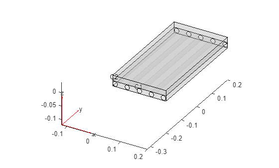
Plot the geometry with the face labels.
figure
pdegplot(g,FaceLabels="on",FaceAlpha=0.2);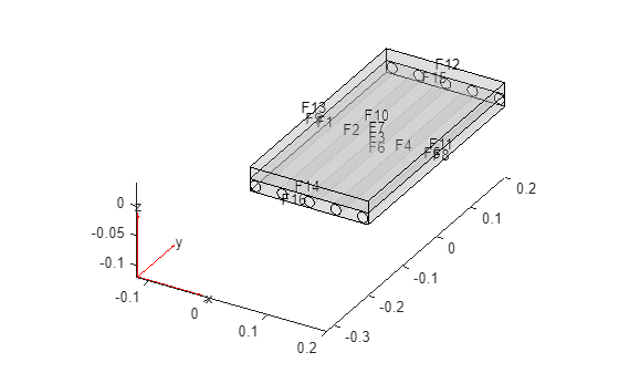
Optimization Problem Setup
Optimize the number of cooling pipes, , and the diameters of the pipes, . All pipes have the same diameter. Search for the number of cooling pipes and their diameters that cause the maximum temperature in the entire geometry to nearly reach, but not exceed, a target temperature in the top block. The objective is the absolute difference between the maximum temperature and the target temperature.
The optimization problem is subject to these constraints:
The temperature at all points in the geometry is no more than the target temperature: .
The number of pipes is between one and nine: .
The pipe diameters are between 0.005 and 0.019: .
To formulate the problem as an optimization problem, place all of the problem variables into one vector . This problem has two optimization variables, and . The variable corresponds to , and the variable corresponds to . Optimization solvers vary the entries in to search for a minimum value of the objective function while maintaining feasibility, which ensures that the constraints are met.
Specify the target temperature and the lower and upper bounds on the number of pipes and their diameters. The lower bound vector lb gives the lower bounds of , which represents the lower bounds of and , which are 1 and 0.005 respectively. The upper bound vector ub represents the upper bounds on and , which are 9 and 0.019 respectively.
Tstar = 358.15;
lb = [1;0.005];
ub = [9;0.019];
Temperature Distribution for Specified Number of Pipes and Pipe Diameter
Create the function that computes temperatures in the cooling plate and the top block based on the number of pipes and their diameters. This function returns the objective function value and the nonlinear constraint function value in the ff.Fval and ff.Ineq fields of the returned structure, ff.
function [ff,results] = ModifyGeomRunFEAforOptim(v,T)
    n = v(1); % number of pipes
    D = v(2); % diameter of each pipe, in meters

    % Specify the length, width, and height of the cooling plate.
    % The top block has the same parameters.
    L = 0.4;% length, in meters
    W = 0.2; % width, in meters
    H = 0.02; % height, same as height of the top block

    % Specify the gap between the edge of the plate and a pipe.
    edgeGap = 1.1*D/2; % in meters

    % Create the stacked cuboids geometry representing the block and the
    % cooling plate.
    g = multicuboid(W,L,[H H],ZOffset=[0 H]);
    g = fegeometry(translate(g,[W/2,0,0]));

    % Create the geometry representing a pipe.
    gCyl = fegeometry(multicylinder(D/2,L));
    gCyl = rotate(gCyl,90,[0 0 0],[1 0 0]);

    % Combine these geometries to represent the top block and the
    % cooling plate with the pipes.
    if n == 1
        gCylT = translate(gCyl,[W/2,L/2,H/2]);
        g = subtract(g,gCylT);
    else
        gPipes = fegeometry;
        for k=linspace(edgeGap,W-edgeGap,n)
            gCylT = translate(gCyl,[k,L/2,H/2]);
            gPipes = union(gPipes,gCylT);
        end
        g=subtract(g,gPipes);
    end

    % Create an femodel object for thermal steady-state analysis and
    % include the geometry into the model.
    model = femodel(AnalysisType="thermalSteady", ...
                    Geometry=g);

    % Specify the thermal conductivity of the cooling plate.
    model.MaterialProperties(1) = ...
        materialProperties(ThermalConductivity=0.5);

    % Specify the thermal conductivity of the top block that produces heat.
    model.MaterialProperties(2) = ...
        materialProperties(ThermalConductivity=80);

    % Specify the heat source in the top block.
    powerWattage = 0.5E3;
    volTopBlock = W*L*H;
    heatSource = powerWattage/volTopBlock;
    model.CellLoad(2) = cellLoad(Heat=heatSource);

    % Compute heat transfer coefficient for convective boundary condition.
    m_dot = 0.02; % mass flow rate, in kg/s
    mu = 0.001002; % dynamic viscosity of water at 293.15K, in kg/(m*s)
    Re = (4*m_dot)/(pi*D*mu); % Reynolds number
    Pr = 7.2; % Prandtl number of water at 293.15K
    if Re >= 10000
        Nu = 0.023*Re^0.8*Pr^0.4; % Nusselt number, use Dittus-Boelter equation for high Re
    else
        Nu = 3.66; % else assume Nu constant
    end
    k = 0.598; % thermal conductivity of water at 293.15K (W/(m*K))
    htc = (Nu*k)/D; % heat transfer coefficient

    % Specify natural convection to ambient on all external faces of the top block
    % and cooling plate. Here, blockFaces are all faces except the pipes and
    % the face between the blocks
    blockFaces = [n+1,(n+3):g.NumFaces];
    model.FaceLoad(blockFaces) = faceLoad(ConvectionCoefficient=20, ...
                                    AmbientTemperature=298.15);

    % Specify forced convection of chilled water in pipes.
    pipeFaces = 1:n;  % faces corresponding to the pipes
    model.FaceLoad(pipeFaces) = faceLoad(ConvectionCoefficient=htc, ...
                                         AmbientTemperature=278.15);
    % Generate a mesh.
    model = generateMesh(model,Hface={pipeFaces,D/5});


    % Solve the model.
    results = solve(model);

    % Find the highest temperature.
    Tmax = max(results.Temperature);

    % Evaluate the objective.
    ff.Fval = abs(T-Tmax);

    % Evaluate the constraints.
    ff.Ineq = Tmax-T;

end
Optimization with surrogateopt
Use the function ModifyGeomRunFEAforOptim as the objective function and nonlinear constraint. Because this objective function is time consuming and the process involves an integer constraint (the number of pipes is an integer), optimize the problem using surrogateopt.
myFun = @(x)ModifyGeomRunFEAforOptim(x,Tstar);
Specify the objective limit for optimization, targetDiff. The optimization process stops when the solution is feasible and the objective function value is no more than targetDiff. The optimization stops when the maximum temperature is less than or equal to the target temperature plus targetDiff.
targetDiff = 0.1;
If you have a Parallel Computing Toolbox™ license, set options to use parallel computing and accelerate the solver. Also set options to stop the solver when the objective function reaches the targetDiff limit.
options = optimoptions("surrogateopt", ...
                       ObjectiveLimit=targetDiff, ...
                       UseParallel=true);
The variable x(1) represents the number of cooling pipes and must be an integer.
intcon = 1;
Run the solver, timing the optimization process. Parallel surrogate optimization is not reproducible, so if you run the solver in parallel, both the timing and the result can vary from run to run. If you run the problem serially, you can ensure reproducibility by setting the random number seed using rng default or a similar statement.
rng default
[sol,fval,flag,output] = surrogateopt(myFun,lb,ub,intcon,options);
Starting parallel pool (parpool) using the 'Processes' profile ... 27-Jan-2026 10:20:01: Job Queued. Waiting for parallel pool job with ID 1 to start ... Connected to parallel pool with 6 workers.
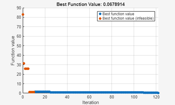
surrogateopt stopped because it exceeded the function evaluation limit set by
'options.MaxFunctionEvaluations'.
Optimal Plate Configuration and Temperature Distribution
Display the optimal number of pipes.
numberOfPipes = sol(1)
numberOfPipes =
7
Display the optimal pipe diameter.
diameterOfPipe = sol(2)
diameterOfPipe =
0.0160
Obtain the solution for the parameters in sol.
[~,results] = ModifyGeomRunFEAforOptim(sol,Tstar);
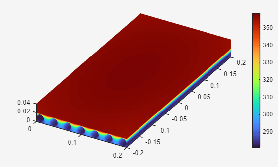
Plot the optimal temperature distribution by using the Visualize PDE Results Live Editor task. First, create a new live script by clicking the New Live Script button in the File section on the Home tab. On the Live Editor tab, select Task > Visualize PDE Results. This action inserts the task into your script. Plot the temperature distribution by following these steps:
In the Select results section of the task, select
resultsfrom the drop-down list.In the Specify data parameters section of the task, set Type to
Temperature.
% Data to visualize
meshData = results.Mesh;
nodalData = results.Temperature;

% Create PDE result visualization
resultViz = pdeviz(meshData,nodalData, ...
"ColorLimits",[280.9 358.2]);
% Clear temporary variables
clearvars meshData nodalData