Eigenvalues and Eigenmodes of L-Shaped Membrane

R2026b

This example shows how to calculate eigenvalues and eigenvectors. The eigenvalue problem is $$-\Delta u=\lambda u$$. This example computes all eigenmodes with eigenvalues smaller than 100.

Create a model and include this geometry. The geometry of the L-shaped membrane is described in the file lshapeg.

model = createpde;
geometryFromEdges(model,@lshapeg);

Set zero Dirichlet boundary conditions on all edges.

applyBoundaryCondition(model,"dirichlet", ...
                       Edge=1:model.Geometry.NumEdges, ...
                       u=0);

Specify the coefficients for the problem: d = 1 and c = 1. All other coefficients are equal to zero.

specifyCoefficients(model,m=0,d=1,c=1,a=0,f=0);

Set the interval [0 100] as the region for the eigenvalues in the solution.

r = [0 100];

Create a mesh and solve the problem.

generateMesh(model,Hmax=0.05);
results = solvepdeeig(model,r);

There are 19 eigenvalues smaller than 100.

length(results.Eigenvalues)

ans = 
19

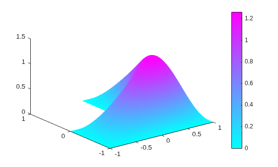
Plot the first eigenmode and compare it to the MATLAB's membrane function.

u = results.Eigenvectors;
pdeplot(model,XYData=u(:,1),ZData=u(:,1));

figure
membrane(1,20,9,9)

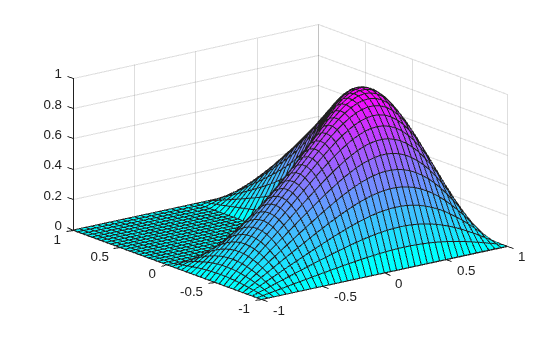
Eigenvectors can be multiplied by any scalar and remain eigenvectors. This explains the difference in scale that you see.

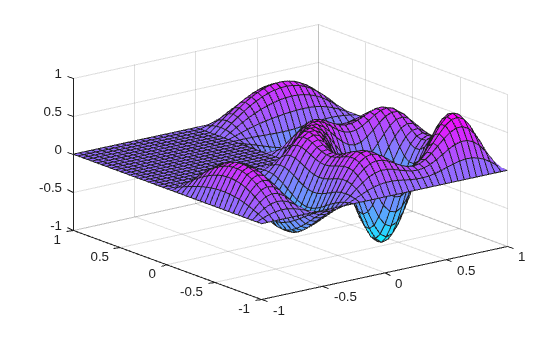
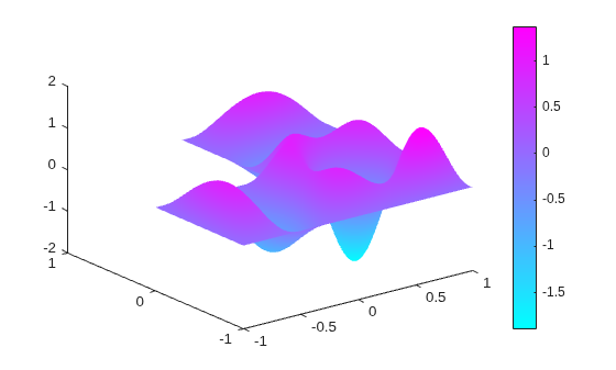
membrane can produce the first 12 eigenfunctions for the L-shaped membrane. Compare the 12th eigenmodes.

figure 
pdeplot(model,XYData=u(:,12),ZData=u(:,12));

figure 
membrane(12,20,9,9)