Passive Bistatic Radar Localization Using OFDM Communication Signals
This example demonstrates a passive bistatic radar system that utilizes a cellular tower as a separate signal source for three-dimensional target localization.
Introduction
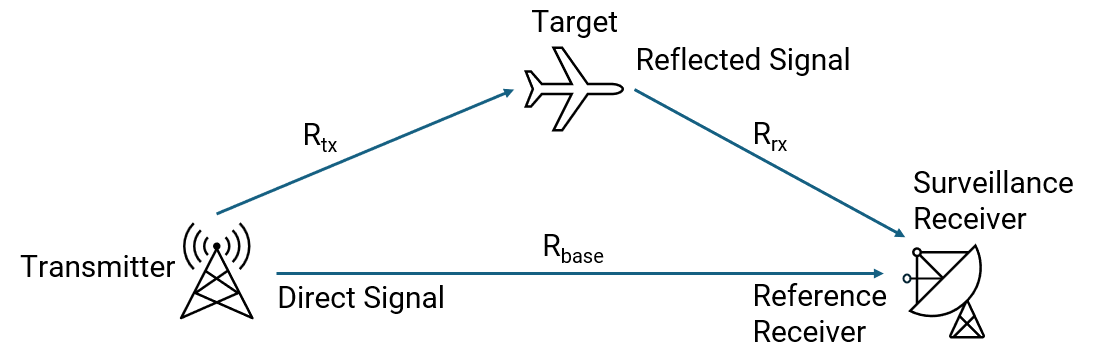
A passive bistatic radar system comprises a separate signal source with a known position, such as a cellular tower, and a passive radar. To accurately localize a target in three-dimensional space, the system requires:
Bistatic Range Measurement: This measurement, , positions the target on an ellipsoid with the transmitter and radar serving as its foci. The range sum represents twice the semi-major axis of this ellipsoid. Because the baseline range —the distance between the transmitter and radar—is known, the range sum can be derived from the bistatic range measurement.
Angle of Arrival (AOA) Measurements: The azimuth and elevation angles of the target's signal observed at the passive radar.
Anchor Positions: The known locations of both the transmitter and the passive radar.
The bistatic range measurement can be obtained through the Time Difference of Arrival (TDOA) between the direct signal and the target-reflected signal. Typically, two receivers are needed at the passive radar to estimate the TDOA. One receiver, known as the reference receiver, is dedicated to capturing the direct signal and often uses a directional antenna pointed directly at the transmitter. The other receiver, called the surveillance receiver, is tasked with collecting the target-reflected signal. The TDOA is determined by performing cross-correlation between the reflected signal received by the surveillance receiver and the direct signal received by the reference receiver.
The AOA measurements, comprising azimuth and elevation angles, indicate the target's direction in three-dimensional space. To estimate the direction of the target's signal, the passive radar employs a two-dimensional array.
The target's position can be estimated by intersecting the target's direction with the ellipsoid defined by the bistatic range measurement. This intersection yields the target's three-dimensional location estimate.
Passive Bistatic Radar System Configuration
Initialize the physical constants required for the simulation.
clear
rng('default')

% RF parameters
fc = 26e9;                                      % Carrier frequency (Hz)
c = physconst('LightSpeed');                    % Speed of propagation (m/s)
bw = 150e6;                                     % Bandwidth (Hz)
fs = bw;                                        % Sample rate (Hz)
lambda = freq2wavelen(fc);                      % Wavelength (m)
Use a short dipole antenna at the transmitter source to transmit signal.
% Configure transmitter
Pt = 10;                                        % Peak power (W)
Gtx = 40;                                       % Tx antenna gain (dB)
transmitter = phased.Transmitter('Gain',Gtx,'PeakPower',Pt);
element = phased.ShortDipoleAntennaElement(AxisDirection = 'Z');
radiator = phased.Radiator('Sensor',element,'OperatingFrequency',fc,'Polarization','Combined');
Utilize a two-dimensional array at the surveillance receiver to capture the target-reflected signal.
% Configure a uniform rectangular array for surveillance receiver
sizeArray = [6 6];
rxarray = phased.URA('Element',element,'Size',sizeArray,'ElementSpacing',[lambda/2,lambda/2]);
numEleRx = getNumElements(rxarray);

% Configure surveillance receiver
Grx = 40;                                       % Rx antenna gain (dB)
NF = 2.9;                                       % Noise figure (dB)
collector = phased.Collector('Sensor',rxarray,'OperatingFrequency',fc,'Polarization','Combined');
receiver = phased.Receiver('AddInputNoise',true,'Gain',Grx, ...
         'NoiseFigure',NF,'SampleRate',fs);
Utilize a directional antenna at the reference receiver to capture the direct signal. This antenna can be designed with the Antenna Toolbox or configured using a polarized antenna element from the Phased Array System Toolbox. In the example code below, a helical antenna is used for the reference receiver if the Antenna Toolbox is licensed. Otherwise, a crossed-dipole antenna is employed.
% Flag to indicate if Antenna Toolbox is licensed useAntennaToolbox =false; if useAntennaToolbox % Configure a helical antenna antenna_ref = design(helix, fc); %#ok<UNRCH> antenna_ref.Tilt = 90; antenna_ref.TiltAxis = [0, 1, 0]; else % Configure a crossed-dipole antenna antenna_ref = phased.CrossedDipoleAntennaElement; end % Configure a conformal array for the reference receiver element_ref = phased.ConformalArray; element_ref.Element = antenna_ref; % Confgure reference receiver collector_ref = phased.Collector('Sensor',element_ref,'OperatingFrequency',fc,'Polarization','Combined'); receiver_ref = clone(receiver);
Platform Configuration
Specify the positions and velocities in transmitter, passive radar, and target platforms.
% Transmitter platform
txpos = [300; 50; -10];                         % Transmitter position (m)
txvel = [0; 0; 0];                              % Transmitter velocity (m/s)
txplatform = phased.Platform('InitialPosition',txpos,'Velocity',txvel,...
    'OrientationAxesOutputPort',true,'OrientationAxes',azelaxes(0,0));

% Passive radar platform
rxpos = [-150; 70; 20];                         % Radar positions (m)
rxvel = zeros(3,1);                             % Radar velocities (m/s)
radarplatform = phased.Platform('InitialPosition',rxpos,'Velocity',rxvel,...
    'OrientationAxesOutputPort',true,'OrientationAxes',azelaxes(0,0));

% Target platform
tgtpos = [80; 40; 110];                         % Target position (m)
tgtvel = [100; 240; 10];                        % Target velocity (m/s)
tgtplatform = phased.Platform('InitialPosition',tgtpos,'Velocity',tgtvel,...
    'OrientationAxesOutputPort',true,'OrientationAxes',azelaxes(0,0));
Specify the clutter positions and velocities in clutter platform.
% Clutter platform clutterpos = [42 -11; 33 -21; 2 -5]; % Clutter position (m) cluttervel = [0.1 -0.2; -0.5 0.3; -0.1 0.15]; % Clutter velocity (m/s) clutterplatform = phased.Platform('InitialPosition',clutterpos,'Velocity',cluttervel,... 'OrientationAxesOutputPort',true,'OrientationAxes',azelaxes(0,0)); % Include clutter in surveillance channels includeClutter =true;
Visualize the bistatic scenario.
helperCreateBistaticScenario(txpos,rxpos,tgtpos,clutterpos,includeClutter);

Obtain target and clutter bistatic range, AOA, and bistatic Doppler ground truth.
[tgtTruth,clutterTruth] = helperBistaticGroundTruth(...
    lambda,txpos,txvel,rxpos,rxvel,tgtpos,tgtvel,clutterpos,cluttervel,includeClutter)
tgtTruth = struct with fields:
BistaticRange: 48.1537
AOA: [2×1 double]
BistaticDoppler: 2.2013e+03
clutterTruth = struct with fields:
      BistaticRange: [3.7550 35.6075]
                AOA: [2×2 double]
    BistaticDoppler: [-11.2474 19.0566]
Channel Configuration
Configure a bistatic channel that comprises both a direct-path channel and a target/clutter-path channel. The direct-path channel refers to the one-way free space channel from the transmitter to the passive radar receiver. In contrast, the target/clutter-path channel involves the transmitter as part of its path.
% One-way free-space propagation channel from the transmitter to passive radar receiver
basechannel = phased.FreeSpace(PropagationSpeed=c,OperatingFrequency=fc, ...
    SampleRate=fs,TwoWayPropagation=false);

% One-way free-space propagation channel from the transmitter to the target
txchannel = clone(basechannel);

% One-way free-space propagation channel from the target to passive radar receiver
rxchannel = clone(basechannel);

% Create a target
smat = 2*eye(2);
target = phased.RadarTarget('PropagationSpeed',c, ...
    'OperatingFrequency',fc,'EnablePolarization',true,...
        'Mode','Bistatic','ScatteringMatrix',smat);

% Create clutters
if includeClutter
    smat_clutter = 5*eye(2);
    numClutter = size(clutterpos,2);
    clutter = cell(1,numClutter);
    for clutterIdx = 1:numClutter
        clutter{clutterIdx} = phased.RadarTarget('PropagationSpeed',c, ...
            'OperatingFrequency',fc,'EnablePolarization',true,...
            'Mode','Bistatic','ScatteringMatrix',smat_clutter);
    end
end
Overview of Signal Processing Chain
The signal processing flow for bistatic radar is outlined below:
Direct-Path Interference and Clutter Cancellation: The surveillance receiver captures not only the target-reflected signal but also direct-path interference and clutter-reflected signals. These unwanted signals typically exhibit low Doppler shifts and can be removed in the Doppler domain using the reference signal.
Bistatic Range Estimation: After canceling interference and clutter, the remaining signal primarily consists of the target-reflected signal. The bistatic range of the target can be estimated by calculating the TDOA between the direct signal and the signal reflected from the target. This estimation can be accomplished by cross-correlating the interference-mitigated signal with the reference signal.
AOA Estimation: on the detected bistatic range bin, array signals are obtained from each element in the two-dimensional surveillance array. These signals are used to estimate the azimuth and elevation angles of the target.
Bistatic Position Estimation: With the bistatic range, azimuth, and elevation angles of the target, a bistatic position estimation algorithm can be employed to determine the target's position.

Please note that this example differs from the "Cooperative Bistatic Radar I/Q Simulation and Processing (Radar Toolbox)" example. The cooperative example demonstrates a collaborative bistatic radar workflow using matched filtering, whereas this example employs a TDOA-based workflow. Additionally, this example focuses on bistatic radar using Orthogonal Frequency-Division Multiplexing (OFDM) communication waveforms, while the cooperative example centers on workflows using collaborative radar waveforms.
Waveform Generation
The cellular tower uses OFDM waveform for signal transmission. Obtain OFDM waveform parameters below.
% Configure OFDM waveform
N = 1024;                                        % Number of subbands (OFDM data carriers)
freqSpacing = bw/N;                              % Frequency spacing (Hz)
tdata = 1/freqSpacing;                           % OFDM data symbol duration (s)
maxDelay = 1.01e-6;                              % Maximum delay (s)
Ncp = ceil(fs*maxDelay);                         % Length of the CP in subcarriers
tcp = Ncp/fs;                                    % Adjusted duration of the CP (s)
tsym = tdata + tcp;                              % OFDM symbol duration (s)
numSample = N + Ncp;                             % Number of subcarriers in one OFDM symbol
The pulse parameters, specifically the pulse repetition interval and the number of pulses, significantly influence the maximum unambiguous Doppler and the resolution in the Doppler domain. These parameters also affect the effectiveness of Doppler-domain interference mitigation. By adjusting the pulse repetition interval and the number of pulses, you can observe their impact on bistatic localization results.
% Pulse paramters
pri = 1.5*tsym;                                  % Pulse repetition interval (s)
numPulse = 128;                                  % Number of pulses
Generate OFDM waveform with modulated data.
% BPSK symbol on each data carrier bpskSymbol = randi([0,1],[N numPulse])*2-1; % Flag to indicate if Communications Toolbox is licensed useCommunicationsToolbox =false; if useCommunicationsToolbox % OFDM modulated signal with cyclic prefix sigmodcp = ofdmmod(bpskSymbol,N,Ncp); %#ok<UNRCH> % Reshape OFDM modulated signal sig = reshape(sigmodcp,N+Ncp,numPulse); else % OFDM symbols with BPSK modulation sigmod = ifft(ifftshift(bpskSymbol,1),[],1); % OFDM symbols with cyclic prefix sig = sigmod([end-Ncp+(1:Ncp),1:end],:); end % Power-normalized OFDM signal sig = sig/max(abs(sig),[],'all');
Radar Data Cubes for Direct-Path Channel
Both the reference receiver and the surveillance receiver capture the direct-path signal from the direct-path channel. Construct the radar data cube containing only the direct-path signal for both the reference and surveillance receivers.
% Radar data cube obtained at reference receiver
Xref = complex(zeros([numSample,1,numPulse]));

% Radar data cube obtained at surveillance receiver
X = complex(zeros([numSample,numEleRx,numPulse]));

% Transmitted signal
txsig = transmitter(sig);

for idxPulse = 1:numPulse
    % Update separate transmitter, radar and target positions
    [tx_pos,tx_vel,tx_ax] = txplatform(pri);
    [radar_pos,radar_vel,radar_ax] = radarplatform(pri);

    % Calculate the transmit angle as seen by the transmitter
    [~,txang_base] = rangeangle(radar_pos,tx_pos,tx_ax);

    % Radiate signal towards the radar receiver
    radtxsig_base = radiator(txsig(:,idxPulse),txang_base,tx_ax);

    % Collect signal at different radar receivers
    % Propagate the signal from the transmitter to each radar
    rxchansig_base = basechannel(radtxsig_base,tx_pos,radar_pos, ...
        tx_vel,radar_vel);

    % Calculate the receive angle
    [~,rxang_base] = rangeangle(tx_pos,radar_pos,radar_ax);

    % Collect signal at the reference receive antenna
    rxsig_ref = collector_ref(rxchansig_base,rxang_base,radar_ax);

    % Receive signal at the reference receiver
    Xref(:,:,idxPulse) = receiver_ref(rxsig_ref);

    % Collect direct-path interference signal at the surveillance
    % receive array
    rxsig_int = collector(rxchansig_base,rxang_base,radar_ax);

    % Receive direct-path interference signal at the surveillance receiver
    X(:,:,idxPulse) = receiver(rxsig_int);
end
reset(txplatform)
reset(radarplatform)
Radar Data Cube for Target/Clutter-Path Channel
The surveillance receiver also captures target-reflected and clutter-reflected signals. Update the radar data cube at the surveillance receiver to incorporate these target-reflected and clutter-reflected signals.
for idxPulse = 1:numPulse
    % Update transmitter, radar and target positions
    [tx_pos,tx_vel,tx_ax] = txplatform(pri);
    [radar_pos,radar_vel,radar_ax] = radarplatform(pri);
    [tgt_pos,tgt_vel,tgt_ax] = tgtplatform(pri);

    % Update clutter positions
    if includeClutter
        [clutter_pos,clutter_vel,clutter_ax] = clutterplatform(pri);
        tgt_pos(:,2:1+numClutter) = clutter_pos;
        tgt_vel(:,2:1+numClutter) = clutter_vel;
        tgt_ax(:,:,2:1+numClutter) = clutter_ax;
    end

    % Calculate the transmit angle for tx-to-target path
    [~,txang] = rangeangle(tgt_pos,tx_pos,tx_ax);

    % Radiate signal towards the target
    radtxsig = radiator(txsig(:,idxPulse),txang,tx_ax);

    % Propagate the signal from the transmitter to the target
    txchansig = txchannel(radtxsig,tx_pos,tgt_pos, ...
        tx_vel,tgt_vel);

    % Reflect the signal off the target
    [~,fwang] = rangeangle(tx_pos,tgt_pos,tgt_ax(:,:,1));
    [~,bckang] = rangeangle(radar_pos,tgt_pos,tgt_ax(:,:,1));
    tgtsig = target(txchansig,fwang,bckang,tgt_ax(:,:,1));

    % Reflect the signal off the clutter
    if includeClutter
        for clutterIdx = 1:numClutter
            [~,fwang] = rangeangle(tx_pos,tgt_pos(:,1+clutterIdx),tgt_ax(:,:,1+clutterIdx));
            [~,bckang] = rangeangle(radar_pos,tgt_pos(:,1+clutterIdx),tgt_ax(:,:,1+clutterIdx));
            tgtsig(1+clutterIdx) = clutter{clutterIdx}(txchansig(1+clutterIdx),fwang,bckang,tgt_ax(:,:,1+clutterIdx));
        end
    end

    % Propagate the signal from the target to each radar
    rxchansig = rxchannel(tgtsig,tgt_pos,radar_pos, ...
        tgt_vel,radar_vel);

    % Calculate the receive angle
    [~,rxang] = rangeangle(tgt_pos,radar_pos,radar_ax);

    % Collect signal at the receive antenna
    rxsig = collector(rxchansig,rxang,radar_ax);

    % Receive signal at the receiver
    X(:,:,idxPulse) = X(:,:,idxPulse) + receiver(rxsig);
end
Clutter and Direct-path Interference Mitigation
Since direct-path interference and clutter-reflected signals exhibit low Doppler shifts, they can be mitigated in the Doppler domain. A widely recognized algorithm for addressing direct-path interference and clutter in bistatic radar is the Enhanced Cancellation Algorithm by Carrier (ECA-C). This algorithm operates by projecting the multi-pulse slow-time signal onto the orthogonal subspace of zero-Doppler.
% Convert time-domain signal in frequency domain
X_freq = fft(X,[],1);
X_freq_ref = fft(Xref,[],1);

% Interference mitigation in slow-time
Xmit_freq = zeros(numSample,numEleRx,numPulse);
for idxSubcarrier = 1:numSample
    % Reference signal over slow-time
    xref_slow = reshape(X_freq_ref(idxSubcarrier,1,:),[numPulse,1]);

    % Projection matrix
    projectMatrix = xref_slow/(xref_slow'*xref_slow)*xref_slow';

    for idxRx = 1:numEleRx
        % Signal in slow-time
        x_slow = reshape(X_freq(idxSubcarrier,idxRx,:),[numPulse,1]);

        % Cancel interference
        Xmit_freq(idxSubcarrier,idxRx,:) = x_slow - projectMatrix*x_slow;
    end
end

% Convert signal back to time-domain
Xmit = ifft(Xmit_freq);
Compare the fast-time signal power before and after mitigation. As illustrated in the figure, the ECA-C algorithm effectively reduces clutter and interference signal power.
% Plot fast-time signal power
pulseIdxPlot = 1;
helperCompareFastTimePower(X,Xmit,pulseIdxPlot)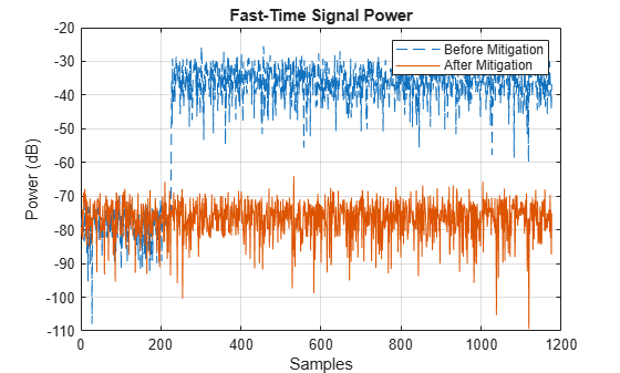
Bistatic Range Estimation
The bistatic range of the target is proportional to the TDOA between the target path and the direct path. The TDOA can be estimated using the phased.TDOAEstimator System object.
% TDOA estimator
numSig = 1;
tdoaestimator = phased.TDOAEstimator(NumEstimates=numSig,...
      SampleRate=fs,TDOAResponseOutputPort=true);

% Estimate bistatic range
for idxPulse = numPulse:-1:1
    % Bistatic data where last dimension has the reference channel and a
    % survelliance channel
    Xtdoa = zeros(numSample,numEleRx,2);
    for rxEleIdx = 1:numEleRx
        % Obtain reference channel signal
        Xtdoa(:,rxEleIdx,1) = Xref(:,1,idxPulse);

        % Obtain survelliance channel signal
        Xtdoa(:,rxEleIdx,2) = Xmit(:,rxEleIdx,idxPulse);
    end

    % Estimate TDOA, get TDOA response and TDOA grid
    [tdoaest,tdoaresp,tdoagrid] = tdoaestimator(Xtdoa);
    tdoaResp(:,:,idxPulse) = tdoaresp;
end

% Convert TDOA to bistatic range
rngest = tdoaest*c;
rnggrid = tdoagrid*c;

% Estimated range indices
rngIndices = zeros(1,numSig);
for estIdx = 1:numSig
    [~,rngIdx] = min(abs(rngest(estIdx)-rnggrid));
    rngIndices(estIdx) = rngIdx;
end

% Plot bistatic range spectrum
helperPlotBistaticRangeSpectrum(tdoaResp,rnggrid,rngIndices,numSig,pulseIdxPlot)
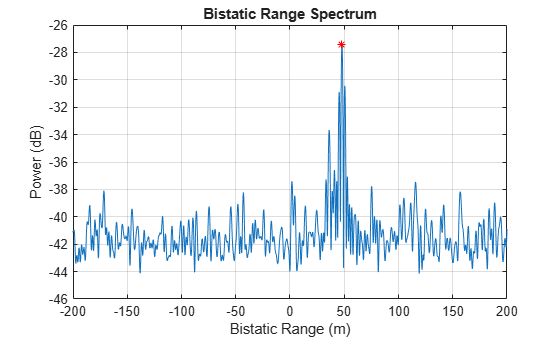
% Bistatic range estimation RMSE
rangermse = rmse(rngest,tgtTruth.BistaticRange);
disp(['RMS bistatic range estimation error = ', num2str(rangermse), ' meters.'])
RMS bistatic range estimation error = 0.1869 meters.
Angle of Arrival Estimation
For the estimated bistatic range bin, determine the azimuth and elevation angles through 2D beam scanning. This can be accomplished using the phased.BeamscanEstimator2D System object.
% Estimate azimuth and elevation of the target
doaestimator = phased.BeamscanEstimator2D(SensorArray=rxarray,...
    OperatingFrequency=fc, ...
    DOAOutputPort=true,NumSignals=numSig,...
    AzimuthScanAngles=-90:1:90,ElevationScanAngles=-90:1:90);
rngIdx = rngIndices(1);
[~,aoaest] = doaestimator(tdoaResp(rngIdx,:,pulseIdxPlot));
figure
plotSpectrum(doaestimator)
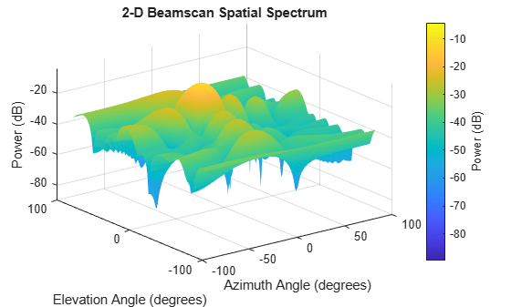
% Angle estimation RMSE
angrmse = rmse(aoaest,tgtTruth.AOA);
disp(['RMS angle estimation error = ', num2str(angrmse), ' degrees.'])
RMS angle estimation error = 0.33839 degrees.
Bistatic Position Estimation
Using the bistatic range estimate along with the azimuth and elevation AOA estimates, the target's 3-D position can be determined with the bistaticposest function.
% Estimate bistatic position
rngmeasurement = 'BistaticRange';
tgtposest = bistaticposest(rngest,aoaest,[],[],txpos,rxpos,...
       RangeMeasurement=rngmeasurement);

% RMSE of target position estimate
rmsepos = rmse(tgtposest,tgtpos);
disp(['RMS positioning error = ', num2str(rmsepos), ' meters.'])
RMS positioning error = 1.6496 meters.
% View position estimate
helperPlotBistaticPositions(rngest,aoaest,tgtposest,txpos,rxpos,tgtpos,rngmeasurement)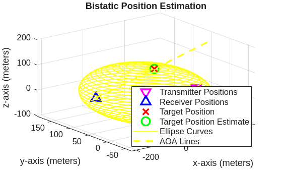
Conclusion
This example illustrates a passive bistatic radar 3-D localization workflow. It covers the simulation of a bistatic radar data cube, the cancellation of direct-path interference and clutter, the estimation of the target's bistatic range, azimuth, and elevation, and the localization of the target using bistatic position estimation.
References
[1] C. Schwark and D. Cristallini, "Advanced multipath clutter cancellation in OFDM-based passive radar systems," 2016 IEEE Radar Conference, Philadelphia, PA, USA, 2016, pp. 1-4.
[2] H. Kuschel, D. Cristallini and K. E. Olsen, "Tutorial: Passive radar tutorial," in IEEE Aerospace and Electronic Systems Magazine, vol. 34, no. 2, pp. 2-19, Feb. 2019.