Use UpdateDetector to Tune Anomaly Detector Performance Without Retraining
This example illustrates different options you can try to tune and improve anomaly detector performance without retraining the detector.
Load the file sineWaveAnomalyData.mat, which contains two sets of synthetic three-channel sinusoidal signals.
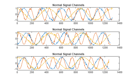
sineWaveNormal contains 10 sinusoids of stable frequency and amplitude. Each signal has a series of small-amplitude impact-like imperfections. The signals have different lengths and initial phases.
load sineWaveAnomalyData.mat sineWaveNormal sineWaveAbnormal
s1 = 3;
Plot input signals
Plot the first three normal signals. Each signal contains three input channels.
tiledlayout("vertical")
ax = zeros(s1,1);
for kj = 1:s1
ax(kj) = nexttile;
    plot(sineWaveNormal{kj})
    title("Normal Signal Channels")
end
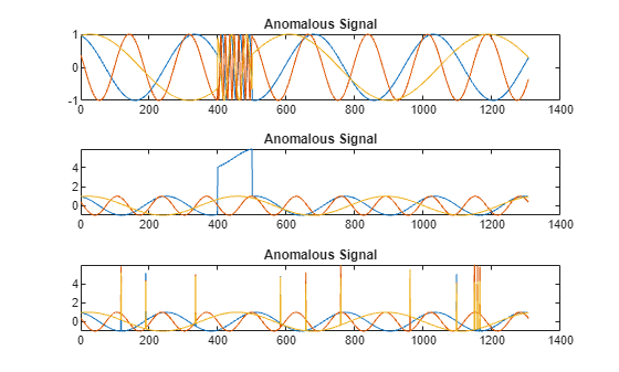
sineWaveAbnormal contains three signals, all of the same length. Each signal in the set has one or more anomalies.
All channels of the first signal have an abrupt change in frequency that lasts for a finite time.
The second signal has a finite-duration amplitude change in one of its channels.
The third signal has spikes at random times in all channels.
Plot the three signals with anomalies.
tiledlayout("vertical")
ax = zeros(s1,1);
for kj = 1:s1
ax(kj) = nexttile;
    plot(sineWaveAbnormal{kj})
    title("Anomalous Signal")
end
Create Detector
Use the USAD function to create a deep learning USAD anomaly detector with default options.
detector_US = usAD(3)
detector_US =
  UsadDetector with properties:

    ObservationWindowLength: 24
      DetectionWindowLength: 24
                      Alpha: 0.7000
                       Beta: 0.3000
             TrainingStride: 24
             LatentSpaceDim: 32
                  IsTrained: 0
                NumChannels: 3
                     Layers: {[7×1 nnet.cnn.layer.Layer]  [7×1 nnet.cnn.layer.Layer]  [7×1 nnet.cnn.layer.Layer]}
                      Dlnet: {[1×1 dlnetwork]  [1×1 dlnetwork]  [1×1 dlnetwork]}
                  Threshold: []
            ThresholdMethod: "kSigma"
         ThresholdParameter: 3
          ThresholdFunction: []
              Normalization: "zscore"
            DetectionStride: 24
Train Detector
Train detector_US using the normal data and the MaxEpochs name-value pair.
detector_US = train(detector_US,sineWaveNormal,MaxEpochs=100);
|======================================================================================|
| Iteration | Epoch |  Time Elapsed  | Base Learning |  AE1 Training  |  AE2 Training  |
|           |       |   (hh:mm:ss)   |      Rate     |      Loss      |     Loss       |
|======================================================================================|
|         1 |     1 |       00:00:00 |        0.0010 |         1.2536 |         1.2550 |
|        50 |    13 |       00:00:04 |        0.0010 |         1.2921 |        -1.1491 |
|       100 |    25 |       00:00:09 |        0.0010 |         1.7565 |        -1.6706 |
|       150 |    38 |       00:00:15 |        0.0010 |         1.9849 |        -1.9378 |
|       200 |    50 |       00:00:20 |        0.0010 |         1.9556 |        -1.9193 |
|       250 |    63 |       00:00:25 |        0.0010 |         1.9973 |        -1.9706 |
|       300 |    75 |       00:00:32 |        0.0010 |         1.9606 |        -1.9383 |
|       350 |    88 |       00:00:36 |        0.0010 |         2.0007 |        -1.9829 |
|       400 |   100 |       00:00:40 |        0.0010 |         1.9641 |        -1.9495 |
|=====================================================================|
Computing threshold...
Threshold computation completed.
View the threshold that train computes and saves within detector_US. This computed value is influenced by random factors, such as which subsets of the data are used for training, and can change somewhat for different training sessions and different machines.
thresh = detector_US.Threshold
thresh =
2.8665
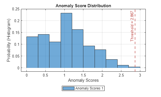
Plot the histogram of the anomaly scores for the normal data. Each score is calculated over a single detection window. The threshold, plotted as a vertical line, does not always completely bound the scores.
plotHistogram(detector_US,sineWaveNormal)
Use Detector to Identify Anomalies
Use the detect function to determine the anomaly scores for the anomalous data.
results = detect(detector_US, sineWaveAbnormal);
results is a cell array that contains three tables, one table for each channel. Each cell table contains three variables: WindowLabel, WindowAnomalyScore, and WindowStartIndices. Confirm the table variable names.
varnames = results{1}.Properties.VariableNamesvarnames = 1×3 cell array
"'Labels'" "'AnomalyScores'" "'StartIndices'"
Plot and Evaluate Results
Plot a histogram that shows the normal data, the anomalous data, and the threshold in one plot.
plotHistogram(detector_US,sineWaveNormal,sineWaveAbnormal)
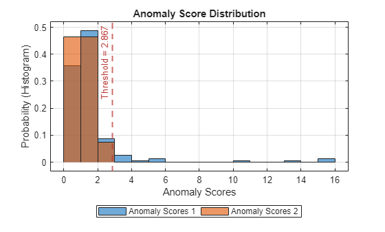
The histogram uses different colors for the normal and anomalous data. The mixed color indicates where the two data sources overlap.
Plot the detected anomalies of the third abnormal signal set.
plot(detector_US,sineWaveAbnormal{3})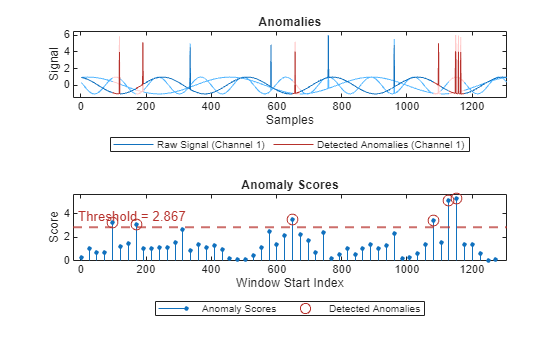
The top plot shows an overlay of red where the anomalies are detected. The blue spikes indicate anomalies that are not detected.
The bottom plot shows that the threshold is too high to capture all the anomalous activity.
Adjust Threshold Manually
Use updateDetector to manually adjust the threshold independently of the input data. The plot of anomaly scores shows that the lowest anomaly scores in the known anomalous region are at about 2.0.
detector_US = updateDetector(detector_US,ThresholdMethod="manual",Threshold=2.0);
results1 = detect(detector_US, sineWaveAbnormal);
plotHistogram(detector_US,sineWaveNormal,sineWaveAbnormal)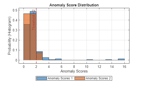
plot(detector_US,sineWaveAbnormal{3})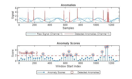
With this threshold, detector_US detects the anomalous region, although there is a little overlap into the healthy portions of the signal.
Change Threshold Method
The default threshold method is "kSigma", and this example uses this method for the initial detector update. Now change the threshold method to "contaminationFraction", which sets the threshold to identify a top percentage of anomaly scores as anomalous, where the percentage is specified in ThresholdParameter. Set ThresholdParameter to 0.05, which results in anomaly identification of the top 5% of the anomaly scores.
detector_US = updateDetector(detector_US,sineWaveNormal,ThresholdMethod="contaminationFraction",ThresholdParameter=0.05);
results2 = detect(detector_US, sineWaveAbnormal);
plotHistogram(detector_US,sineWaveNormal,sineWaveAbnormal)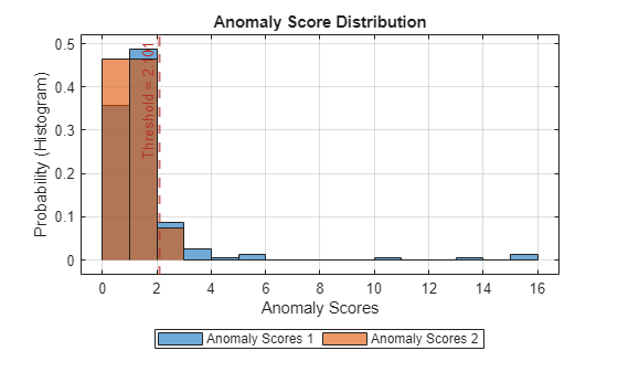
This approach yields a similar result to setting the threshold manually.
plot(detector_US,sineWaveAbnormal{3})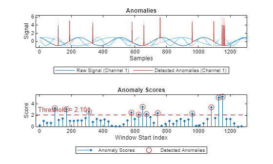
This approach performs similarly to the manual threshold adjustment.
Modify Model Tuning Parameters
For a USAD model, you can modify the tuning parameters alpha and beta without invalidating the original detector training. These parameters must sum to 1. The default values are 0.7 and 0.3, respectively. Use updateDetector to change alpha and beta to 0.9 and 0.1. Also, restore the original threshold method to the "kSigma" and threshold parameter to 3.
detector_US = updateDetector(detector_US,sineWaveNormal,ThresholdMethod="kSigma",ThresholdParameter=3,Alpha=0.9,Beta=0.1);
results3 = detect(detector_US, sineWaveAbnormal);
plotHistogram(detector_US,sineWaveNormal,sineWaveAbnormal)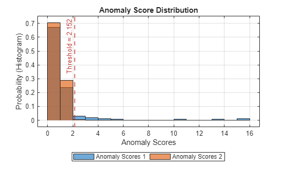
plot(detector_US,sineWaveAbnormal{3})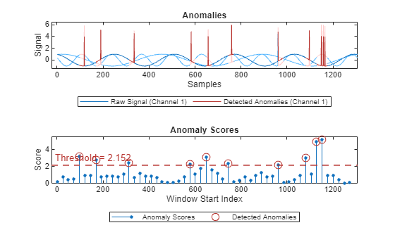
In this case the performance is better than the original anomaly detection with the same threshold method / parameter, but with different values for Alpha and Beta.
Test Detector on Other Signals
The detector performs well on Signal 3. Now test the detector against abnormal Signals 1 and 2.
plot(detector_US,sineWaveAbnormal{1})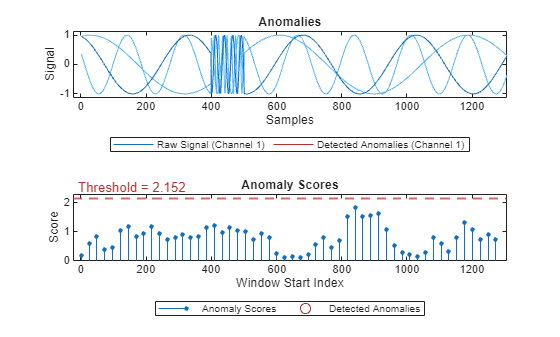
plot(detector_US,sineWaveAbnormal{2})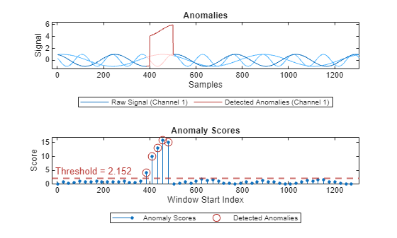
detectorUS does not perform well on Signal 1, but does perform well on Signal 2.
Copyright 2026 The MathWorks, Inc