Estimate Expected Shortfall with the expectedShortfall Function

This example shows how to calculate expected shortfall (ES) estimates for a normally distributed portfolio returns distribution by using the expectedShortfall function in Risk Management Toolbox™. ES, a market risk metric, supplements the value-at-risk (VaR) by estimating the average potential loss in value of a portfolio on the percentage of days when the VaR is violated.

In this example, you first compute the ES values by using the expectedShortfall function. Then, you compare those values against ES values that you compute by an analytical formula, by averaging VaR values, and by averaging inverted cumulative distribution function (CDF) values.

Compute ES Using expectedShortfall

First, load a volatility data set.

load('ESBacktestDistributionData.mat','NormalStd');

Next, set a VaR level and use the expectedShortfall function to compute the ES values for a normal distribution with a mean of 0 and a standard deviation contained in the variable NormalStd. Use the string "normal" to specify a normal distribution.

VaRLevel = .95;
ES = expectedShortfall("normal",VaRLevel,Mean=0,StandardDeviation=NormalStd);

Compute ES from Analytical Formula

The analytical formula [1] for calculating ES for a portfolio returns distribution that follows a normal distribution is:

${\text{ES}}_{\alpha }={\sigma }_{\text{portfolio}}\left(\frac{\varphi \left({\Phi }^{-1}\left(\alpha \right)\right)}{1-\alpha }\right)-{\mu }_{\text{portfolio}}$,

where:

${\mu }_{\text{portfolio}}$ is the mean portfolio return (assumed 0).

${\sigma }_{\text{portfolio}}$ is the standard deviation of the portfolio returns.

$\alpha$ is the confidence level (.95).

$\varphi$ is the probability distribution function (PDF) for the normal distribution.

$\Phi$ is the CDF of the normal distribution.

Set a VaR level and compute ES estimates using this formula:

mu = 0;
VaRLevel = .95;
esByAnalyticFormula = -1*(mu-NormalStd*normpdf(norminv(VaRLevel))./(1-VaRLevel));

Then, compare the output from expectedShortfall against the analytical formula. The plots are identical because the expectedShortfall function uses the analytical formula. This answer is the most accurate and provides the best performance in comparison with averaging VaR values and averaging inverted CDF values.

X = 1:length(NormalStd);
f = figure;
plot(X, ES, 'b.', X, esByAnalyticFormula,'r-');
xlabel('Trading Day')
ylabel('ES Value')
legend({'ES from expectedShortfall','ES from analytical formula'},'Location','Best')

Compute ES from Average of VaR Values

You can also calculate VaR estimates for different thresholds above 95% and then estimate the tail average (the ES of the portfolio distribution) by averaging the VaR values in the tail. An ES estimate is the probability-weighted average of tail losses and is calculated from the VaR threshold. For example, given a 95% VaR for a portfolio, you must average the tail losses from the 95th–100th percentile to calculate the associated ES value. One way to estimate the ES for a given VaR value is to average a set of VaR values with a greater confidence level [2]. For this example, the 95% VaR is the primary VaR, but you can also calculate the VaR for the confidence levels from 95.5% to 99.5% in increments of 0.5%. Then, estimate the ES for the 95% VaR by averaging these higher VaR values.

First, create a grid of confidence levels greater than 95%.

esVaRLevels = [0.955, 0.96, 0.965, 0.97, 0.975, 0.98, 0.985, 0.99, 0.995];

To calculate VaR values, use the valueAtRisk function. For a normal distribution, specify "normal" for the first input argument. Use the loaded volatilities to calculate the VaR values for the grid of VaRLevels, assuming a normal returns distribution with a mean of 0 and a standard deviation given by NormalStd.

esVaRValues = valueAtRisk("normal",esVaRLevels,Mean=0,StandardDeviation=NormalStd); 

Average the computed VaR estimates by using the mean function to get ES estimates.

esByVaRAverage = mean(esVaRValues,2);

Compute ES from Average of Inverted Normal CDF Values

An alternative approach you can use is to derive VaR values from a normal probability distribution function (PDF) and calculate the VaR values by inverting the CDF for the normal PDF that is defined by the VaR method. Consider the following CDF and PDF. createNormalCDFandPDF is a helper function that generates the plots shown next.

createNormalCDFandPDF;

The top plot depicts the portfolio returns CDF with a selected set of equally spaced y-values going from 0 to $1-\alpha ,$ where $\alpha$ is the confidence level, in this case, from 0 to 0.05. You can invert the y-values to get a set of x-values, which represent portfolio returns (losses) over the relevant portion of the PDF. Because the y-values represent probability thresholds, and are equally spaced, a simple average gives the probability-weighted average of the tail of the PDF. This is equivalent to calculating a set of equally spaced VaR values and averaging them.

The bottom plot depicts the portfolio returns PDF along with a set of y-values equivalent to the y-values in the top plot. These values are not equally spaced, but if they were, a simple average of the x-values would not yield the probability-weighted average of the tail losses. Instead, you have to weight each x-value with a point estimate of the probability of the *x-*value (an estimate of the area under the curve between the lines). However, because the specified y-values are equally spaced in probability, a simple average yields the correct answer.

In these two plots, the CDF and PDF distributions assume a mean of 0 and a variance of 1. The VaR methodology also assumes a mean of 0 and saves the volatility estimates for each day in the vector NormalStd. Using this value, you can estimate the ES as an average of inverted normal CDF values.

To perform averaging of inverted normal CDF values, first create a grid of probabilities from 0 to 0.05. Invert the CDFs for each volatility estimate and each probability by using norminv. Average these values over the probabilities to get ES estimates for each trading day.

p = .0001:.0001:.05;
mu = 0;
invertedNormValues = -norminv(p,mu,NormalStd);
esByInvertedNormalCDF = mean(invertedNormValues,2);

Compare Results for ES Methods

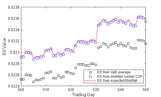
Plot the ES values versus trading day from the expectedShortfall function, from averaging VaR values, and from averaging inverted CDF values. The plots show that these values are similar and esByVaRAverage consistently comes in lowest. The VaR average uses only nine VaR values, which misses a larger fraction of the tail of the returns distribution compared to the other methods. Because the largest losses are farther along the tail, this results in a slightly lower ES estimate.

X = 1:length(NormalStd);
f = figure;
plot(X, esByVaRAverage, 'ks', X, esByInvertedNormalCDF, 'bo', X, ES,'r-');
xlabel('Trading Day')
ylabel('ES Value')
legend({'ES from VaR average','ES from inverted normal CDF','ES from expectedShortfall'},'Location','Best')
xlim([500 550])

ES Options

The method that expectedShortfall uses to calculate the ES value varies depending on the type of distribution you provide as input to the function. You can specify "normal", "t", or "empirical" for the distribution. The expectedShortfall function uses an ES formula to calculate values for each of these distribution types.

You can also specify a probability distribution object for the distribution input argument when you use expectedShortfall. The four types of probability distribution objects you can choose from are:

• Normal distribution

• t location-scale distribution

• Piecewise linear distribution

• Kernel distribution

For normal and t location-scale distributions, expectedShortfall extracts the parameters and calculates the ES output using the associated formula. For piecewise linear and kernel distributions, expectedShortfall uses the CDF inversion method. This means the output ES value is a numerical approximation, and the performance varies depending on the number of VaRLevels, the number of trading days, the size of the tail that expectedShortfall needs to estimate (the tail is larger for a 95% VaR than for a 99% VaR), the type of distribution (piecewise linear is significantly faster than kernel), and the number of observations within the distribution. For more details about using this function, see expectedShortfall.

References

[1] McNeil, Alexander J., Rüdiger Frey, and Paul Embrechts. Quantitative Risk Management: Concepts, Techniques and Tools. Princeton Series in Finance. Princeton, N.J: Princeton University Press, 2005.

[2] Dowd, Kevin. Measuring Market Risk. 1st ed. Wiley, 2005.