skyplot

R2026b

Plot satellite azimuth and elevation data

Syntax

skyplot(azdata,eldata)

skyplot(azdata,eldata,labeldata)

skyplot(status)

skyplot(___,Name,Value)

skyplot(parent,___)

h = skyplot(___)

Description

skyplot(azdata,eldata) creates a sky plot using the azimuth and elevation data specified as matrices in degrees. Azimuth angles are measured in degrees, clockwise-positive from the North direction. Elevation angles are measured from the horizon line with 90 degrees being directly up. For details about the sky plot figure elements, see Main Sky Plot Elements.

skyplot(azdata,eldata,labeldata) specifies data labels as a string array with elements corresponding to each data point in the azdata and eldata inputs.

skyplot(status) specifies the azimuth and elevation data in a structure with fields SatelliteAzimuth and SatelliteElevation.

skyplot(___,Name,Value) specifies options using one or more name-value arguments in addition to the input arguments in previous syntaxes. The name-value arguments are properties of the SkyPlotChart object. For a list of properties, see SkyPlotChart Properties.

skyplot(parent,___) creates the sky plot in the figure, panel, or tab specified by parent.

h = skyplot(___) returns the sky plot as a SkyPlotChart object, h. Use h to modify the properties of the chart after creating it. For a list of properties, see SkyPlotChart Properties.

Examples

View Satellite Positions from GNSS Sensor

Create a GNSS sensor model as a gnssSensor (Navigation Toolbox) System object™.

gnss = gnssSensor; 

Specify the position and velocity of the sensor. Simulate the sensor readings and get status from visible satellites. Store the azimuth and elevation angles as vectors.

pos = [0 0 0]; 
vel = [0 0 0]; 
[~, ~, status] = gnss(pos, vel); 
satAz = status.SatelliteAzimuth; 
satEl = status.SatelliteElevation; 

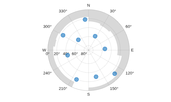
Create random local elevation masks, with a maximum elevation of 30 degrees, to act as the local environment.

rng(8)
terrainMaskElevations = 30*rand(1,12); % elevations (degrees)
terrainMaskEdges = [0 24 48 100 132 180 204 240 276 288 300 312 360]; % azimuth edges (degrees)

Plot the satellite positions with the elevation masks.

skyplot(satAz,satEl,MaskElevation=terrainMaskElevations,MaskAzimuthEdges=terrainMaskEdges); 

Plot Series of Satellite Positions over Time

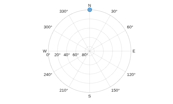
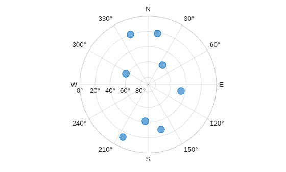
Animate the trajectory of satellite positions over time from a GNSS sensor.

Initialize the sky plot figure. Specify the relevant time-stepping information.

skyplotHandle = skyplot(0,0); 

numHours = 12; 
dt = 100; 
numSeconds = numHours * 60 * 60; 
numSimSteps = numSeconds/dt;

Create a GNSS sensor model as a gnssSensor (Navigation Toolbox) System Object™.

gnss = gnssSensor('SampleRate', 1/dt); 

Iterate through the time steps and do the following:

• Simulate the sensor readings. Specify the zero position and velocity for the stationary sensor.

• Store the azimuth and elevation angles as vectors.

• Set the AzimuthData and ElevationData properties of the SkyPlotChart handle directly.

for i = 1:numSimSteps 

    [~, ~, status] = gnss([0 0 0],[0 0 0]); 

    satAz = status.SatelliteAzimuth; 
    satEl = status.SatelliteElevation; 

    set(skyplotHandle,'AzimuthData',satAz,'ElevationData',satEl);
    
    drawnow 
end 

View Satellite Positions for Different Groups

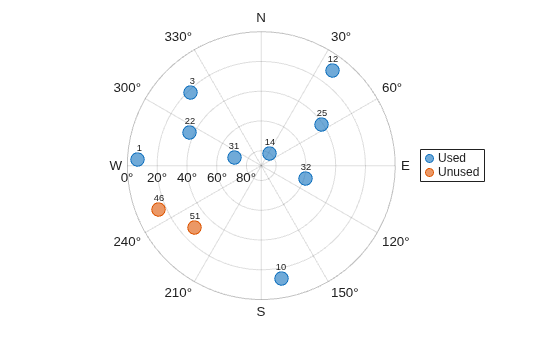
Load the azimuth and elevation data from a logfile generated by an Adafruit® GPS satellite sensor. The data provided in this example contains the azimuth and elevation of each satellite and the pseudorandom noise (PRN) codes. Store these values as vectors.

load('gpsHWInfo','hwInfo') 
satAz = hwInfo.SatelliteAzimuths; 
satEl = hwInfo.SatelliteElevations; 
prn = hwInfo.SatellitePRNs; 

Separate the satellites based on the PRN codes. To correlate each position with a group, create a categorical array. For this set of satellites, only the ones with PRNs less than 32 are used in the positioning solution.

isUnused = (prn > 32);
group = categorical(isUnused,[false true],["Used in Positioning Solution" "Unused"]);

Visualize the satellites and specify the categorical groups in the GroupData name-value argument. Specify the PRN as the label for each point. Show the legend.

skyplot(satAz,satEl,prn,GroupData=group) 
legend('Used','Unused')

Visualize Satellite Trajectories in Skyplot

Specify the receiver position, RINEX navigation file, mask angle, time step size, and number of hours of data to sample from the RINEX file.

recPos = [42 -71 50];
navfile = "GODS00USA_R_20211750000_01D_GN.rnx";
maskAngle = 25;
dt = 60; % seconds
numHours = 2;

Read the navigation file, and get the GPS data of all satellites captured in the file.

data = rinexread(navfile);
[~,satIdx] = unique(data.GPS.SatelliteID);
navmsg = data.GPS(satIdx,:);

Set the starting time to the initial time of the navigation message. Then, create the time vector t.

startTime = navmsg.Time(1);
secondsPerHour = 3600;
timeElapsed = 0:dt:(secondsPerHour*numHours);
t = startTime + seconds(timeElapsed);

Initialize vectors for azimuth and elevation. Then, collect azimuth and elevation data at times t for all satellites.

numSats = numel(navmsg.SatelliteID);
allAz = NaN(numel(t),numSats);
allEl = allAz;
for idx = 1:numel(t)
    [satPos,~,satID] = gnssconstellation(t(idx),RINEXData=navmsg);
    [az,el,vis] = lookangles(recPos,satPos,maskAngle);
    allAz(idx,:) = az;
    allEl(idx,:) = el;
end

Mark all satellites below the horizon with an elevation less than 0 as missing.

allEl(allEl < 0) = missing;

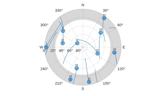
Display the satellite trajectories as an animation by creating a skyplot and updating the AzimuthData and ElevationData properties.

figure
sp = skyplot(allAz(1,:),allEl(1,:),satID,MaskElevation=maskAngle);
for idx = 1:size(allAz, 1)
    set(sp,AzimuthData=allAz(1:idx,:),ElevationData=allEl(1:idx,:));
    drawnow limitrate
end

Model Obstructions with Elevation Mask

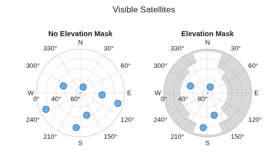
Specify a custom elevation mask to model the effect of nearby buildings on satellite visibility. In this scenario, the receiver is positioned on a city road, with higher obstructions to the east and west.

recPos = [42 -71 50];
maskAngles = [5 35 50 25 5 25 35 25 5];
azEdges = [0 20 40 140 160 200 220 320 340 360];

Set the observation time and obtain satellite positions for that instant.

t = datetime(2025,10,1);
satPos = gnssconstellation(t);

Determine which satellites are visible, first without any mask, then apply the elevation mask to represent the urban obstructions.

[az,el,visMask] = lookangles(recPos,satPos,maskAngles,azEdges);
[az,el,visNoMask] = lookangles(recPos,satPos);

Visualize the results by comparing satellite visibility with and without the elevation mask.

t1 = tiledlayout(1,2);
title(t1,"Visible Satellites");

nexttile
skyplot(az(visNoMask),el(visNoMask))
title("No Elevation Mask")

nexttile
skyplot(az(visMask),el(visMask),MaskElevation=maskAngles,MaskAzimuthEdges=azEdges)
title("Elevation Mask")

Color Satellite Trajectories by Signal Strength

Color the satellite trajectories on a sky plot by a time-varying quantity, such as received signal strength, by using the ColorData property of skyplot.

Read the satellite signal strength from a RINEX observation file and the Galileo navigation data from the corresponding navigation file.

obsData = rinexread("GODS00USA_R_20211750000_01H_30S_MO.rnx");
navData = rinexread("GODS00USA_R_20211750000_01D_EN.rnx");
galObs  = obsData.Galileo;

Pair the Galileo observations with the broadcast ephemeris by using gnssmeasurements, which returns each satellite position row-aligned to the observation table.

meas = gnssmeasurements(galObs,navData.Galileo,"C1X");

Estimate the receiver position from the measurements by using receiverposition, which returns one latitude-longitude-altitude estimate per time stamp. Because this receiver is a stationary ground station, average the per-epoch estimates to obtain a single, more robust position that smooths out measurement noise.

recPos = mean(receiverposition(meas),1);

Convert the satellite positions to azimuth and elevation look angles relative to the receiver, and read the E1 signal strength S1X (carrier-to-noise density, in dB-Hz).

[az,el] = lookangles(recPos,meas.SatellitePosition);
signal  = galObs.S1X;

The ColorData property must be the same size as the azimuth and elevation data, with one row per time stamp and one column per satellite. Reshape the row-aligned vectors onto that grid.

t   = unique(galObs.Time);
ids = unique(galObs.SatelliteID);
[~,row] = ismember(galObs.Time,t);
[~,col] = ismember(galObs.SatelliteID,ids);
sz = [numel(t) numel(ids)];
azimuth   = accumarray([row col],az,sz,[],NaN);
elevation = accumarray([row col],el,sz,[],NaN);
strength  = accumarray([row col],signal,sz,[],NaN);

Plot the satellite trajectories, coloring them by signal strength with the ColorData property. Label the colorbar with the signal strength units.

sp = skyplot(azimuth,elevation,string(ids),ColorData=strength);
sp.Colormap      = parula;
sp.ColorbarLabel = "Signal Strength C/N_0 (dB-Hz)";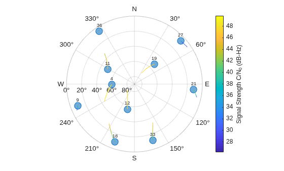

Input Arguments

azdata — Azimuth angles for visible satellite positions

n-element vector of angles | t-by-n matrix of angles

Azimuth angles for visible satellite positions, specified as an n-element vector of angles or t-by-n matrix of angles. n is the number of visible satellite positions in the plot, and t is the number of time steps of the satellites. Azimuth angles are measured in degrees, clockwise-positive from the north direction, and must be in the range [0, 360].

Example: [25 45 182 356] specifies the azimuth angles for four satellites at one time step.

s

Data Types: double

eldata — Elevation angles for visible satellite positions

n-element vector of angles | t-by-n matrix of angles

Elevation angles for visible satellite positions, specified as an n-element vector of angles or t-by-n matrix of angles. n is the number of visible satellite positions in the plot, and t is the number of time steps of the satellites. Elevation angles are measured from the horizon line with 90 degrees being directly up and must be in the range [MinElevation, 90].

Example: [45 90 27 74] specifies the elevation angles for four satellites at one time step.

Data Types: double

labeldata — Labels for visible satellite positions

n-element string array

Labels for visible satellite positions, specified as an n-element string array. n is the number of visible satellite positions in the plot.

Example: ["G1" "G11" "G7" "G3"]

Data Types: string

status — Satellite status

structure | structure array

Satellite status, specified as a structure or structure array. Satellite status structures contain the fields SatelliteAzimuth and SatelliteElevation. Typically, this status structure comes from a gnssSensor (Navigation Toolbox) object, which simulates satellite positions and velocities.

Example: gnss = gnssSensor; [~,~,status] = gnss(position,velocity)

Data Types: struct

parent — Parent container

Figure object | Panel object | Tab object | TiledChartLayout object | GridLayout object

Parent container, specified as a Figure, Panel, Tab, TiledChartLayout, or GridLayout object.

Output Arguments

h — Sky plot chart

SkyPlotChart object

Sky plot chart, returned as a SkyPlotChart object, which is a standalone visualization. Use h to set properties on the sky plot chart. For more information, see SkyPlotChart Properties (Navigation Toolbox).

More About

Main Sky Plot Elements

The main elements of the figure are:

• Azimuth axes — Specified by the azdata input argument, azimuth angle positions are measured clockwise-positive from the North direction and are in the range [0, 360].

• Elevation axes —Specified by the eldata input argument, elevation angle positions are measured from the horizon line with 90 degrees being directly up and are in the range [MinElevation, 90].

• Labels — Specified by the labeldata input argument as a string array with an element for each point in the azdata and eldata vectors.

• Groups — Specified by the GroupData (Navigation Toolbox) property, a categorical array defines the group for each satellite position.

Standalone Visualization

A standalone visualization is a chart designed for a special purpose that works independently from other charts. Unlike other charts such as plot and surf, a standalone visualization has a preconfigured axes object built into it, and some customizations are not available. A standalone visualization also has these characteristics:

• It cannot be combined with other graphics elements, such as lines, patches, or surfaces. Thus, the hold command is not supported.

• The gca function can return the chart object as the current axes.

• You can pass the chart object to many MATLAB^® functions that accept an axes object as an input argument. For example, you can pass the chart object to the title function.

Version History

Introduced in R2021a

R2026b: Visualize time-varying metrics along satellite trajectories with enhanced color support

You can now visualize time-varying metrics along satellite trajectories using color scaling with these new SkyPlotChart properties:

• TrajectoryColor

• ColorData

• Colormap

• ColorScaling

• ColorLimits

• ColorLimitsMode

• ColorbarLabel

• ColorbarVisible

This enhancement allows you to represent time-varying satellite characteristics like carrier-to-noise ratio directly on trajectories.

R2026b: Visualize satellites at negative elevation angles

You can now visualize satellites at negative elevation angles by specifying a minimum elevation using the new MinElevation property of SkyPlotChart. This enhancement helps you analyze satellite visibility for high-altitude observers, such as Low Earth Orbit (LEO) scenarios, where satellites below the horizon are relevant.

R2024b: Specify the status of multiple satellites

The status argument now additionally accepts structure arrays to specify the status of more than one satellite.

R2022b: skyplot supports azimuth and elevation trajectories and elevation masks

• The azdata and eldata arguments now accept matrices, enabling you to represent trajectories by adding azimuth and elevation data for satellites at multiple time steps.

• Elevation angle masks are now supported using these new SkyPlotChart properties:

  • MaskElevation (Navigation Toolbox)

  • MaskAlpha (Navigation Toolbox)

  • MaskColor (Navigation Toolbox)

  • MaskAzimuthEdges (Navigation Toolbox)

  • MaskAzimuthEdgesMode (Navigation Toolbox)