pburg

Autoregressive power spectral density estimate — Burg’s method

Syntax

pxx = pburg(x,order)

pxx = pburg(x,order,nfft)

[pxx,w] = pburg(___)

[pxx,f] = pburg(___,Fs)

[pxx,w] = pburg(x,order,w)

[pxx,f] = pburg(x,order,f,Fs)

[___] = pburg(x,order,___,freqRange)

[___,pxxc] = pburg(___,ConfidenceLevel=p)

pburg(___)

Description

pxx = pburg(x,order) returns the power spectral density (PSD) estimate, pxx, of a discrete-time signal, x, found using Burg’s method. When x is a vector, it is treated as a single channel. When x is a matrix, the PSD is computed independently for each column and stored in the corresponding column of pxx. pxx is the distribution of power per unit frequency. The frequency is expressed in units of rad/sample. order is the order of the autoregressive (AR) model used to produce the PSD estimate.

pxx = pburg(x,order,nfft) uses nfft points in the discrete Fourier transform (DFT). For real x, pxx has length (nfft/2+1) if nfft is even, and (nfft+1)/2 if nfft is odd. For complex–valued x, pxx always has length nfft. If you omit nfft, or specify it as empty, then pburg uses a default DFT length of 256.

[pxx,w] = pburg(___) returns the vector of normalized angular frequencies, w, at which the PSD is estimated. w has units of rad/sample. For real-valued signals, w spans the interval [0,π] when nfft is even and [0,π) when nfft is odd. For complex-valued signals, w always spans the interval [0,2π).

[pxx,f] = pburg(___,Fs) returns a frequency vector, f, in cycles per unit time. The sample rate, Fs, is the number of samples per unit time. If the unit of time is seconds, then f is in cycles/second (Hz). For real-valued signals, f spans the interval [0,Fs/2] when nfft is even and [0,Fs/2) when nfft is odd. For complex-valued signals, f spans the interval [0,Fs). Fs must be the fourth input to pburg. To input a sample rate and still use the default values of the preceding optional arguments, specify these arguments as empty, [].

[pxx,w] = pburg(x,order,w) returns the two-sided AR PSD estimates at the normalized frequencies specified in the vector, w. The vector w must contain at least two elements, because otherwise the function interprets it as nfft.

[pxx,f] = pburg(x,order,f,Fs) returns the two-sided AR PSD estimates at the frequencies specified in the vector, f. The vector f must contain at least two elements, because otherwise the function interprets it as nfft. The frequencies in f are in cycles per unit time. The sample rate, Fs, is the number of samples per unit time. If the unit of time is seconds, then f is in cycles/second (Hz).

[___] = pburg(x,order,___,freqRange) returns the AR PSD estimate over the frequency range specified by freqRange. Valid options for freqRange are: "onesided", "twosided", or "centered".

[___,pxxc] = pburg(___,ConfidenceLevel=p) returns the p × 100% confidence intervals for the PSD estimate in pxxc.

pburg(___) with no output arguments plots the AR PSD estimate in dB per unit frequency in the current figure window.

Examples

Burg PSD Estimate of an AR(4) Process

Create a realization of an AR(4) wide-sense stationary random process. Estimate the PSD using Burg's method. Compare the PSD estimate based on a single realization to the true PSD of the random process.

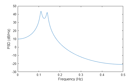
Create an AR(4) system function. Obtain the frequency response and plot the PSD of the system.

A = [1 -2.7607 3.8106 -2.6535 0.9238];
[H,F] = freqz(1,A,[],1);
plot(F,mag2db(abs(H)))

xlabel("Frequency (Hz)")
ylabel("PSD (dB/Hz)")

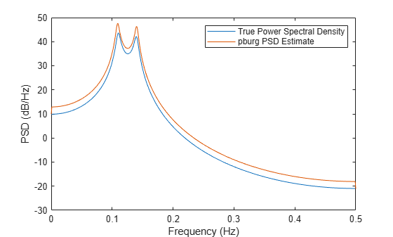
Create a realization of the AR(4) random process. Set the random number generator to the default settings for reproducible results. The realization is 1000 samples in length. Assume a sample rate of 1 Hz. Use pburg to estimate the PSD for a 4th-order process. Compare the PSD estimate with the true PSD.

rng("default")

x = randn(1000,1);
y = filter(1,A,x);
[Pxx,F] = pburg(y,4,1024,1);

hold on
plot(F,pow2db(Pxx))
legend(["True Power Spectral Density" "pburg PSD Estimate"])

Reflection Coefficients for Model Order Determination

Create a realization of an AR(4) process. Use arburg to determine the reflection coefficients. Use the reflection coefficients to determine an appropriate AR model order for the process. Obtain an estimate of the process PSD.

Create a realization of an AR(4) process 1000 samples in length. Reset the random number generator for reproducible results.

rng("default")

A = [1 -2.7607 3.8106 -2.6535 0.9238];
x = filter(1,A,randn(1000,1));

Use arburg with the order set to 12 to return the reflection coefficients. Plot the reflection coefficients to determine an appropriate model order.

[a,e,k] = arburg(x,12);

stem(k,"filled")
title("Reflection Coefficients")
xlabel("Model Order")

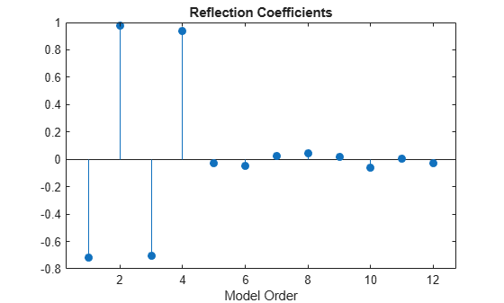
The reflection coefficients decay to zero after order 4. This response indicates that an AR(4) model is most appropriate.

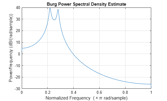
Obtain a PSD estimate of the random process using Burg's method. Use 1000 points in the DFT. Plot the PSD estimate.

pburg(x,4,length(x))

Burg PSD Estimate of a Multichannel Signal

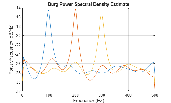
Create a multichannel signal consisting of three sinusoids in additive $$N(0,1)$$ white Gaussian noise. Reset the random number generator for reproducible results. The sinusoids frequencies are 100 Hz, 200 Hz, and 300 Hz. The sample rate is 1 kHz, and the signal has a duration of 1 second.

rng("default")
Fs = 1000;
t = 0:1/Fs:1-1/Fs;
f = [100;200;300];

x = cos(2*pi*f*t)' + randn(length(t),3);

Estimate the PSD of the signal using Burg's method with a 12th-order autoregressive model. Use the default DFT length. Plot the estimate.

mOrder = 12;

pburg(x,mOrder,[],Fs)

Input Arguments

x — Input signal

vector | matrix

Input signal, specified as a vector or as a matrix. If you specify x as a matrix, then pburg treats its columns as independent channels.

Example: cos(pi/4*(0:159))+randn(1,160) is a single-channel row-vector signal.

Example: cos(pi./[4;2]*(0:159))'+randn(160,2) is a two-channel signal.

Data Types: single | double
Complex Number Support: Yes

order — Order of autoregressive model

positive integer

Order of the autoregressive model, specified as a positive integer.

Data Types: double

nfft — Number of DFT points

256 (default) | integer | []

Number of DFT points, specified as a positive integer. For a real-valued input signal, x, the PSD estimate, pxx has length (nfft/2+1) if nfft is even, and (nfft+1)/2 if nfft is odd. For a complex-valued input signal,x, the PSD estimate always has length nfft. If nfft is specified as empty, the default nfft is used.

Data Types: single | double

Fs — Sample rate

positive scalar

Sample rate, specified as a positive scalar. The sample rate is the number of samples per unit time. If the unit of time is seconds, then the sample rate is in Hz.

• If you specify Fs as empty [], then pburg assumes that the input signal x has a sample rate of 1 Hz.

• If you do not specify Fs, then pburg assumes that the input signal x has a sample rate of 2π rad/sample.

w — Normalized frequencies

vector

Normalized frequencies, specified as a row or column vector with at least two elements. Normalized frequencies are in rad/sample.

Example: w = [pi/4 pi/2]

Data Types: double | single

f — Frequencies

vector

Frequencies, specified as a row or column vector with at least two elements. The frequencies are in cycles per unit time. The unit time is specified by the sample rate, fs. If fs has units of samples/second, then f has units of Hz.

Example: fs = 1000; f = [100 200]

Data Types: double | single

freqRange — Frequency range for PSD estimate

"onesided" | "twosided" | "centered"

Frequency range of the PSD estimate, specified as "onesided", "twosided", or "centered".

The pburg function returns pxx with a number of rows and frequency interval that depends on the value specified in freqRange, whether the number of DFT points freqSpec is even or odd, and whether Fs is specified or not.

freqRange	freqSpec	Number of Rows in pxx	Frequency Interval for pxx
			Fs unspecified	Fs specified
"onesided" (default if x is real-valued)	Even	freqSpec/2 + 1	[0,π] rad/sample	[0,Fs/2] cycles/unit time
	Odd	(freqSpec + 1)/2	[0,π) rad/sample	[0,Fs/2) cycles/unit time
"twosided" (default if x is complex-valued)	Even or odd	freqSpec	[0,2π) rad/sample	[0,Fs) cycles/unit time
"centered"	Even	freqSpec	(–π,π] rad/sample	(–Fs/2,Fs/2] cycles/unit time
	Odd		(–π,π) rad/sample	(–Fs/2,Fs/2) cycles/unit time

Note

• This argument is not supported if you specify freqSpec as a vector of cyclical or normalized frequencies.

• If you specify the "onesided" value, pburg multiplies the power by 2 at all frequencies except 0 and the Nyquist frequency to conserve the total power.

• The "onesided" value is not supported if x is complex-valued.

Data Types: char | string

p — Confidence interval for PSD estimate

0.95 (default) | scalar in the range (0,1)

Coverage probability for the PSD estimate, specified as a scalar in the range (0,1).

If you specify ConfidenceLevel=p and pxxc, the function outputs pxxc with the lower and upper bounds of the p × 100% interval estimate for the true PSD.

Output Arguments

pxx — PSD estimate

vector | matrix

PSD estimate, returned as a real-valued, nonnegative column vector or matrix.

• Each column of pxx is the PSD estimate of the corresponding column of x.

• The units of the PSD estimate are in squared-magnitude units of the input signal per unit frequency. For example, if the input data x is in volts, you specify the sample rate Fs in hertz, and you assume a resistance of 1 Ω, then the PSD estimate is in watts per hertz.

w — Normalized frequencies

vector

Normalized frequencies, returned as a real-valued column vector. If pxx is a one-sided PSD estimate, w spans the interval [0,π] if nfft is even and [0,π) if nfft is odd. If pxx is a two-sided PSD estimate, w spans the interval [0,2π). For a DC-centered PSD estimate, w spans the interval (–π,π] for even nfft and (–π,π) for odd nfft.

f — Cyclical frequencies

vector

Cyclical frequencies, returned as a real-valued column vector. For a one-sided PSD estimate, f spans the interval [0,fs/2] when nfft is even and [0,fs/2) when nfft is odd. For a two-sided PSD estimate, f spans the interval [0,fs). For a DC-centered PSD estimate, f spans the interval (–fs/2, fs/2] cycles/unit time for even length nfft and (–fs/2, fs/2) cycles/unit time for odd length nfft.

pxxc — Confidence bounds

matrix

Confidence bounds, returned as a real-valued matrix.

• pxxc has the same number of rows as in pxx.

• pxxc has twice as many columns as pxx.

  • Odd-numbered columns contain the lower bounds of the confidence intervals.

  • Even-numbered columns contain the upper bounds of the confidence intervals.

  Thus, pxxc(m,2*n-1) is the lower confidence bound and pxxc(m,2*n) is the upper confidence bound corresponding to the estimate pxx(m,n).

• The coverage probability of the confidence intervals is determined by the value of the p input.

Data Types: single | double

Extended Capabilities

C/C++ Code Generation

Generate C and C++ code using MATLAB® Coder™.

Usage notes and limitations:

If the nfft argument is variable-size at compile time, then it must not become a scalar or an empty array at runtime.

GPU Code Generation

Generate CUDA® code for NVIDIA® GPUs using GPU Coder™.

Refer to the usage notes and limitations in the C/C++ Code Generation section. The same usage notes and limitations apply to GPU code generation.

Version History

Introduced before R2006a