plotActualVersusPredicted
Compare predictions to actual data, creating a subplot for each response
Description
plotActualVersusPredicted(
shows the comparison between predictions to the actual data, with a subplot for each
response.resultsObj)
Examples
Load the sample data set.
load data10_32R.mat
gData = groupedData(data);
gData.Properties.VariableUnits = ["","hour","milligram/liter","milligram/liter"];
Create a two-compartment PK model.
pkmd                 = PKModelDesign;
pkc1                 = addCompartment(pkmd,"Central");
pkc1.DosingType      = "Infusion";
pkc1.EliminationType = "linear-clearance";
pkc1.HasResponseVariable = true;
pkc2                 = addCompartment(pkmd,"Peripheral");
model                = construct(pkmd);
configset            = getconfigset(model);
configset.CompileOptions.UnitConversion = true;
responseMap = ["Drug_Central = CentralConc","Drug_Peripheral = PeripheralConc"];
Provide model parameters to estimate.
paramsToEstimate   = ["log(Central)","log(Peripheral)","Q12","Cl_Central"];
estimatedParam     = estimatedInfo(paramsToEstimate,'InitialValue',[1 1 1 1]);
Assume every individual receives an infusion dose at time = 0, with a total infusion amount of 100 mg at a rate of 50 mg/hour.
dose             = sbiodose("dose","TargetName","Drug_Central");
dose.StartTime   = 0;
dose.Amount      = 100;
dose.Rate        = 50;
dose.AmountUnits = "milligram";
dose.TimeUnits   = "hour";
dose.RateUnits   = "milligram/hour";
Estimate model parameters. By default, the function estimates a set of parameter for each individual (unpooled fit).
fitResults = sbiofit(model,gData,responseMap,estimatedParam,dose);
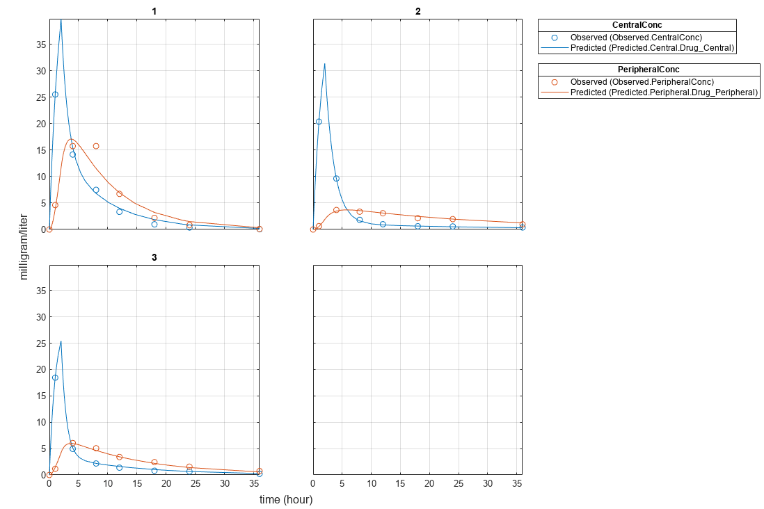
Plot the results.
plot(fitResults);
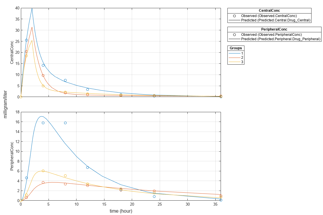
Plot all groups in one plot.
plot(fitResults,"PlotStyle","one axes");
Change some axes properties.
s = struct;
s.Properties.XGrid = "on";
s.Properties.YGrid = "on";
plot(fitResults,"PlotStyle","one axes","AxesStyle",s);

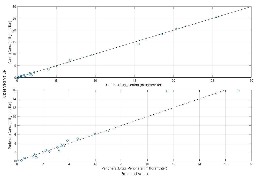
Compare the model predictions to the actual data.
plotActualVersusPredicted(fitResults)
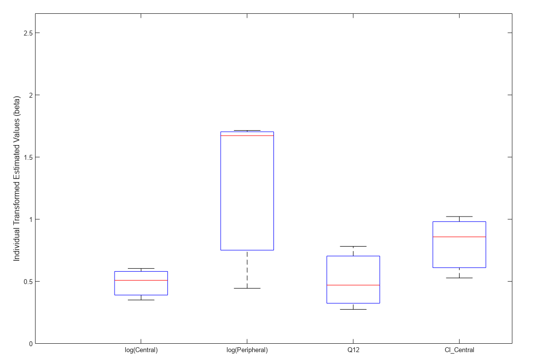
Use boxplot to show the variation of estimated model parameters.
boxplot(fitResults)
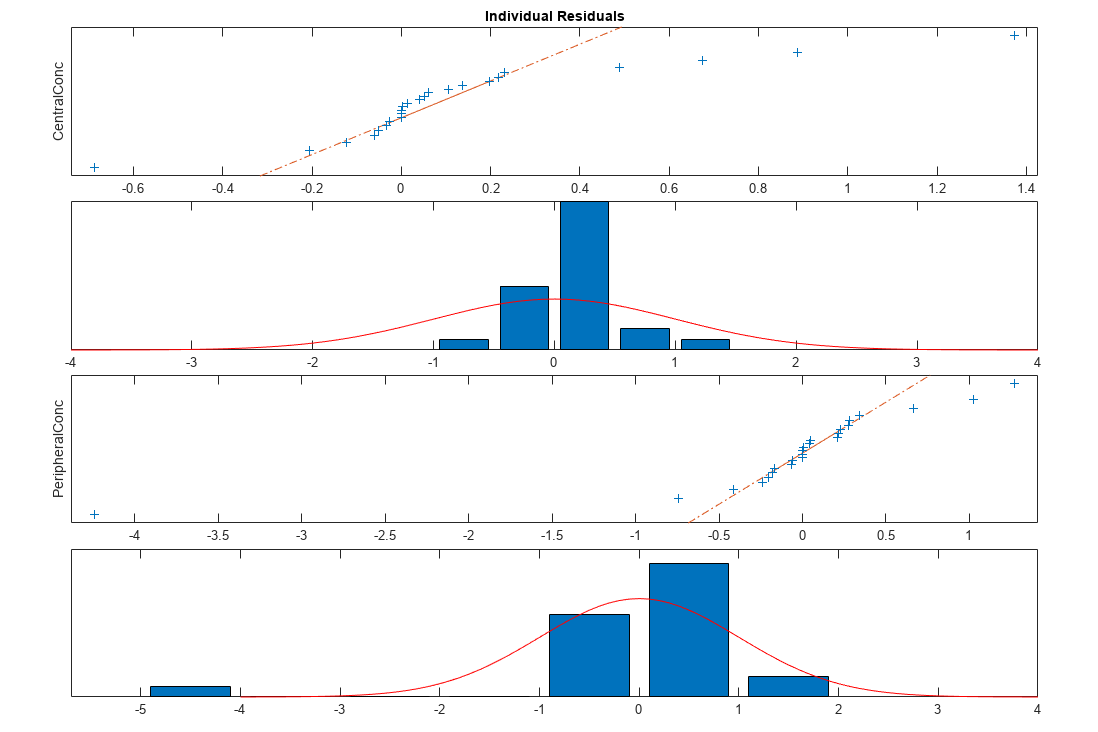
Plot the distribution of residuals. This normal probability plot shows the deviation from normality and the skewness on the right tail of the distribution of residuals. The default (constant) error model might not be the correct assumption for the data being fitted.
plotResidualDistribution(fitResults)
Plot residuals for each response using the model predictions on x-axis.
plotResiduals(fitResults,"Predictions")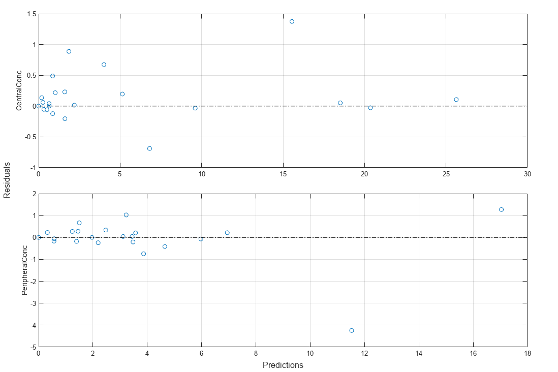
Get the summary of the fit results. stats.Name contains the name for each table from stats.Table, which contains a list of tables with estimated parameter values and fit quality statistics.
stats = summary(fitResults);
stats.Name
ans =
'Unpooled Parameter Estimates'
ans =
'Statistics'
ans =
'Unpooled Beta'
ans =
'Residuals'
ans =
'Covariance Matrix'
ans =
'Error Model'
stats.Table
ans=3×9 table
    Group    Central Estimate    Central StandardError    Peripheral Estimate    Peripheral StandardError    Q12 Estimate    Q12 StandardError    Cl_Central Estimate    Cl_Central StandardError
    _____    ________________    _____________________    ___________________    ________________________    ____________    _________________    ___________________    ________________________

    {'1'}          1.422                0.12334                 1.5619                   0.36355               0.47163            0.15196                0.5291                  0.036978
    {'2'}         1.8322               0.019672                 5.3364                   0.65327                0.2764           0.030799               0.86035                  0.026257
    {'3'}         1.6657               0.038529                 5.5632                   0.37063               0.78361           0.058657                1.0233                  0.027311
ans=3×7 table
    Group      AIC        BIC      LogLikelihood    DFE      MSE         SSE
    _____    _______    _______    _____________    ___    ________    _______

    {'1'}     60.961     64.051       -26.48        12        2.138     25.656
    {'2'}    -7.8379    -4.7475       7.9189        12     0.029012    0.34814
    {'3'}    -1.4336     1.6567       4.7168        12     0.043292     0.5195
ans=3×9 table
    Group    Central Estimate    Central StandardError    Peripheral Estimate    Peripheral StandardError    Q12 Estimate    Q12 StandardError    Cl_Central Estimate    Cl_Central StandardError
    _____    ________________    _____________________    ___________________    ________________________    ____________    _________________    ___________________    ________________________

    {'1'}        0.35208               0.086736                 0.44589                   0.23277              0.47163            0.15196                0.5291                  0.036978
    {'2'}        0.60551               0.010737                  1.6746                   0.12242               0.2764           0.030799               0.86035                  0.026257
    {'3'}        0.51027                0.02313                  1.7162                  0.066621              0.78361           0.058657                1.0233                  0.027311
ans=24×4 table
    ID    Time    CentralConc    PeripheralConc
    __    ____    ___________    ______________

    1       0              0               0
    1       1        0.10646        -0.74394
    1       4         1.3745          1.2726
    1       8       -0.68825         -4.2435
    1      12        0.67383         0.21806
    1      18        0.88823          1.0269
    1      24        0.48941         0.66755
    1      36        0.13632         0.22948
    2       0              0               0
    2       1      -0.026731       -0.058311
    2       4      -0.033299        -0.20544
    2       8       -0.20466         0.20696
    2      12       -0.12223        0.045409
    2      18       0.041224         0.33883
    2      24      -0.059498       0.0036257
    2      36      -0.051645         0.27616
      ⋮
ans=12×6 table
    Group      Parameters        Central      Peripheral        Q12        Cl_Central
    _____    ______________    ___________    __________    ___________    ___________

    {'1'}    {'Central'   }       0.015213     -0.022539     -0.0086672       0.001159
    {'1'}    {'Peripheral'}      -0.022539       0.13217       0.045746     -0.0073135
    {'1'}    {'Q12'       }     -0.0086672      0.045746       0.023092     -0.0021484
    {'1'}    {'Cl_Central'}       0.001159    -0.0073135     -0.0021484      0.0013674
    {'2'}    {'Central'   }     0.00038701     -0.002161    -0.00010177     9.7448e-05
    {'2'}    {'Peripheral'}      -0.002161       0.42676       0.019101      -0.015755
    {'2'}    {'Q12'       }    -0.00010177      0.019101     0.00094857    -0.00073328
    {'2'}    {'Cl_Central'}     9.7448e-05     -0.015755    -0.00073328     0.00068942
    {'3'}    {'Central'   }      0.0014845    -0.0054648     -0.0013216     0.00016639
    {'3'}    {'Peripheral'}     -0.0054648       0.13737       0.016903     -0.0072722
    {'3'}    {'Q12'       }     -0.0013216      0.016903      0.0034406    -0.00082538
    {'3'}    {'Cl_Central'}     0.00016639    -0.0072722    -0.00082538     0.00074587
ans=3×5 table
    Group     Response      ErrorModel        a        b
    _____    __________    ____________    _______    ___

    {'1'}    {0×0 char}    {'constant'}     1.2663    NaN
    {'2'}    {0×0 char}    {'constant'}    0.14751    NaN
    {'3'}    {0×0 char}    {'constant'}    0.18019    NaN
Input Arguments
Version History
Introduced in R2014a