MATLAB Workflow for Tuning the HL-20 Autopilot
This is Part 5 of the example series on design and tuning of the flight control system for the HL-20 vehicle. This part shows how to perform most of the design in MATLAB® without interacting with the Simulink® model.
Background
This example uses the HL-20 model adapted from NASA HL-20 Lifting Body Airframe (Aerospace Blockset), see Part 1 of the series (Trimming and Linearization of the HL-20 Airframe) for details. The autopilot controlling the attitude of the aircraft consists of three inner loops and three outer loops.

In Part 2 (Angular Rate Control in the HL-20 Autopilot) and Part 3 (Attitude Control in the HL-20 Autopilot - SISO Design), we showed how to close the inner loops and tune the gain schedules for the outer loops. These examples made use of the slTuner interface to interact with the Simulink model, obtain linearized models and control system responses, and push tuned values back to Simulink.
For simple architectures and rapid design iterations, it can be preferable (and conceptually simpler) to manipulate the linearized models in MATLAB and use basic commands like feedback to close loops. This example shows how to perform the design steps of Parts 2 and 3 in MATLAB.
Obtaining the Plant Models
To tune the autopilot, we need linearized models of the transfer function from deflections to angular position and rates. To do this, start from the results from the "Trim and Linearize" step (see Trimming and Linearization of the HL-20 Airframe). Recall that G7 is a seven-state linear model of the airframe at 40 different (alpha,beta) conditions, and CS is the linearization of the Controls Selector block.
load csthl20_TrimData G7 CS
Using the Simulink model "csthl20_trim" as reference for selecting I/Os, build the desired plant models by connecting G7 and CS in series. Do not forget to convert phi,alpha,beta from radians to degrees.
r2d = 180/pi;
G = diag([1 1 1 r2d r2d r2d]) * G7([4:7 31:32],1:6) * CS(:,1:3);

G.InputName = {'da','de','dr'};
G.OutputName = {'p','q','r','Phi_deg','Alpha_deg','Beta_deg'};

size(G)
8x5 array of state-space models. Each model has 6 outputs, 3 inputs, and 7 states.
This gives us an array of plant models over the 8-by-5 grid of (alpha,beta) conditions used for trimming.
Closing the Inner Loops
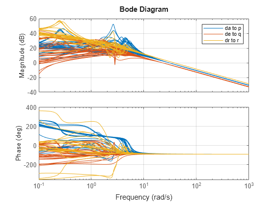
To close the inner loops, we follow the same procedure as in Part 2 (Angular Rate Control in the HL-20 Autopilot). This consists of selecting the gain Kp,Kq,Kr to set the crossover frequency of the p,q,r loops to 30, 22.5, and 37.5 rad/s, respectively.
% Compute Kp,Kq,Kr for each (alpha,beta) condition.
Gpqr = G({'p','q','r'},:);
Kp = 1./abs(evalfr(Gpqr(1,1),30i));
Kq = -1./abs(evalfr(Gpqr(2,2),22.5i));
Kr = -1./abs(evalfr(Gpqr(3,3),37.5i));

bode(Gpqr(1,1)*Kp,Gpqr(2,2)*Kq,Gpqr(3,3)*Kr,{1e-1,1e3}), grid
legend('da to p','de to q','dr to r')

Use feedback to close the three inner loops. Insert an analysis point at the plant inputs da,de,dr for later evaluation of the stability margins.
Cpqr = append(ss(Kp),ss(Kq),ss(Kr));
APu = AnalysisPoint('u',3);  APu.Location = {'da','de','dr'};

Gpos = feedback(G * APu * Cpqr, eye(3), 1:3, 1:3);
Gpos.InputName = {'p_demand','q_demand','r_demand'};

size(Gpos)
8x5 array of generalized state-space models.
Each model has 6 outputs, 3 inputs, 7 states, and 1 blocks.
Note that these commands seamlessly manage the fact that we are dealing with arrays of plants and gains corresponding to the various (alpha,beta) conditions.
Tuning the Outer Loops
Next move to the outer loops. We already have an array of linear models Gpos for the "plant" seen by the outer loops. As done in Part 3 (Attitude Control in the HL-20 Autopilot - SISO Design), parameterize the six gain schedules as polynomial surfaces in alpha and beta. Again we use quadratic surfaces for the proportional gains and multilinear surfaces for the integral gains.
% Grid of (alpha,beta) design points
alpha_vec = -10:5:25;	 % Alpha Range
beta_vec = -10:5:10;     % Beta Range
[alpha,beta] = ndgrid(alpha_vec,beta_vec);
SG = struct('alpha',alpha,'beta',beta);

% Proportional gains
alphabetaBasis = polyBasis('canonical',2,2);
P_PHI = tunableSurface('Pphi', 0.05, SG, alphabetaBasis);
P_ALPHA = tunableSurface('Palpha', 0.05, SG, alphabetaBasis);
P_BETA = tunableSurface('Pbeta', -0.05, SG, alphabetaBasis);

% Integral gains
alphaBasis = @(alpha) alpha;
betaBasis = @(beta) abs(beta);
alphabetaBasis = ndBasis(alphaBasis,betaBasis);
I_PHI = tunableSurface('Iphi', 0.05, SG, alphabetaBasis);
I_ALPHA = tunableSurface('Ialpha', 0.05, SG, alphabetaBasis);
I_BETA = tunableSurface('Ibeta', -0.05, SG, alphabetaBasis);
The overall controller for the outer loop is a diagonal 3-by-3 PI controller taken the errors on angular positions phi,alpha,beta and calculating the rate demands p_demand,q_demand,r_demand.
KP = append(P_PHI,P_ALPHA,P_BETA);
KI = append(I_PHI,I_ALPHA,I_BETA);
Cpos = KP + KI * tf(1,[1 0]);
Finally, use feedback to obtain a tunable closed-loop model of the outer loops. To enable tuning and closed-loop analysis, insert analysis points at the plant outputs.
RollOffFilter = tf(10,[1 10]);
APy = AnalysisPoint('y',3);  APy.Location = {'Phi_deg','Alpha_deg','Beta_deg'};

T0 = feedback(APy * Gpos(4:6,:) * RollOffFilter * Cpos ,eye(3));
T0.InputName = {'Phi_demand','Alpha_demand','Beta_demand'};
T0.OutputName = {'Phi_deg','Alpha_deg','Beta_deg'};
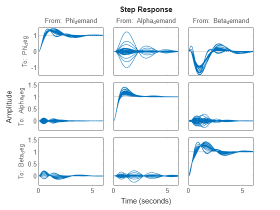
You can plot the closed-loop responses for the initial gain surface settings (constant gains of 0.05).
step(T0,6)

Tuning Goals
Use the same tuning goals as in Part 3 (Attitude Control in the HL-20 Autopilot - SISO Design). These include "MinLoopGain" and "MaxLoopGain" goals to set the gain crossover of the outer loops between 0.5 and 5 rad/s.
R1 = TuningGoal.MinLoopGain({'Phi_deg','Alpha_deg','Beta_deg'},0.5,1);
R1.LoopScaling = 'off';
R2 = TuningGoal.MaxLoopGain({'Phi_deg','Alpha_deg','Beta_deg'},tf(50,[1 10 0]));
R2.LoopScaling = 'off';
These also include a varying "Margins" goal to impose adequate stability margins in each loop and across loops.
% Gain margins vs (alpha,beta)
GM = [...
   6     6     6     6     6
   6     6     7     6     6
   7     7     7     7     7
   7     7     7     7     7
   7     7     7     7     7
   7     7     7     7     7
   6     6     7     6     6
   6     6     6     6     6];

% Phase margins vs (alpha,beta)
PM = [...
   40         40          40         40        40
   40         40          45         40        40
   45         45          45         45        45
   45         45          45         45        45
   45         45          45         45        45
   45         45          45         45        45
   40         40          45         40        40
   40         40          40         40        40];

% Create varying goal
FH = @(gm,pm) TuningGoal.Margins({'da','de','dr'},gm,pm);
R3 = varyingGoal(FH,GM,PM);
Gain Schedule Tuning
You can now use systune to shape the six gain surfaces against the tuning goals at all 40 design points.
T = systune(T0,[R1 R2 R3]);
Final: Soft = 1.03, Hard = -Inf, Iterations = 53
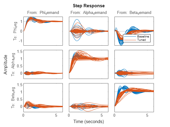
The final objective value is close to 1 so the tuning goals are essentially met. Plot the closed-loop angular responses and compare with the initial settings.
step(T0,T,6)
legend('Baseline','Tuned','Location','SouthEast')

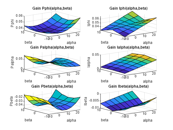
The results match those obtained in Parts 2 and 3. The tuned gain surfaces are also similar.
clf
% NOTE: setBlockValue updates each gain surface with the tuned coefficients in T
subplot(3,2,1), viewSurf(setBlockValue(P_PHI,T))
subplot(3,2,3), viewSurf(setBlockValue(P_ALPHA,T))
subplot(3,2,5), viewSurf(setBlockValue(P_BETA,T))
subplot(3,2,2), viewSurf(setBlockValue(I_PHI,T))
subplot(3,2,4), viewSurf(setBlockValue(I_ALPHA,T))
subplot(3,2,6), viewSurf(setBlockValue(I_BETA,T))
You could now use evalSurf to sample the gain surfaces and update the lookup tables in the Simulink model. You could also use the codegen method to generate code for the gain surface equations. For example
% Generate code for "P phi" block
MCODE = codegen(setBlockValue(P_PHI,T));

% Get tuned values for the "I phi" lookup table
Kphi = evalSurf(setBlockValue(I_PHI,T),alpha_vec,beta_vec);