Linearize Nonlinear Models

What Is Linearization?

Linearization is a linear approximation of a nonlinear system that is valid in a small region around an operating point.

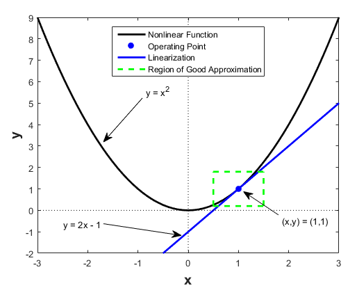
For example, suppose that the nonlinear function is $y = x^{2}$ . Linearizing this nonlinear function about the operating point x = 1, y = 1 results in a linear function $y = 2 x - 1$ .

Near the operating point, $y = 2 x - 1$ is a good approximation to $y = x^{2}$ . Away from the operating point, the approximation is poor.

The next figure shows a possible region of good approximation for the linearization of $y = x^{2}$ . The actual region of validity depends on the nonlinear model.

Extending the concept of linearization to dynamic systems, you can write continuous-time nonlinear differential equations in this form:

$\begin{array}{l} \dot{x} (t) = f (x (t), u (t), t) \\ y (t) = g (x (t), u (t), t) . \end{array}$

In these equations, x(t) represents the system states, u(t) represents the inputs to the system, and y(t) represents the outputs of the system.

A linearized model of this system is valid in a small region around the operating point t=t₀, x(t₀)=x₀, u(t₀)=u₀, and y(t₀)=g(x₀,u₀,t₀)=y₀.

To represent the linearized model, define new variables centered about the operating point:

$\begin{array}{l} δ x (t) = x (t) - x_{0} \\ δ u (t) = u (t) - u_{0} \\ δ y (t) = y (t) - y_{0} \end{array}$

The linearized model in terms of δx, δu, and δy is valid when the values of these variables are small:

$\begin{array}{l} δ \dot{x} (t) = A δ x (t) + B δ u (t) \\ δ y (t) = C δ x (t) + D δ u (t) \end{array}$

Applications of Linearization

Linearization is useful in model analysis and control design applications.

Exact linearization of the specified nonlinear Simulink^® model produces linear state-space, transfer-function, or zero-pole-gain equations that you can use to:

Plot the Bode response of the Simulink model.
Evaluate loop stability margins by computing open-loop response.
Analyze and compare plant response near different operating points.
Design linear controller
Classical control system analysis and design methodologies require linear, time-invariant models. Simulink Control Design™ automatically linearizes the plant when you tune your compensator. See Choose a Control Design Approach.
Analyze closed-loop stability.
Measure the size of resonances in frequency response by computing closed-loop linear model for control system.
Generate controllers with reduced sensitivity to parameter variations and modeling errors.

Linearization in Simulink Control Design

You can use Simulink Control Design software to linearize continuous-time, discrete-time, or multirate Simulink models. The resulting linear time-invariant model is in state-space form.

By default, Simulink Control Design linearizes models using a block-by-block approach. This block-by-block approach individually linearizes each block in your Simulink model and combines the results to produce the linearization of the specified system.

You can also linearize your system using full-model numerical perturbation, where the software computes the linearization of the full model by perturbing the values of the root-level inputs and states. For each input and state, the software perturbs the model by a small amount and computes a linear model based on the model response to these perturbations. You can perturb the model using either forward differences or central differences.

The block-by-block linearization approach has several advantages to full-model numerical perturbation:

Most Simulink blocks have a preprogrammed linearization that provides an exact linearization of the block.
You can use linear analysis points to specify a portion of the model to linearize.
You can configure blocks to use custom linearizations without affecting your model simulation.
Structurally nonminimal states are automatically removed.
You can specify linearizations that include uncertainty (requires Robust Control Toolbox™ software).
You can obtain detailed diagnostic information.
When linearizing multirate models, you can use different rate conversion methods. Full-model numerical perturbation can only use zero-order-hold rate conversion.

Model Requirements for Exact Linearization

Exact linearization supports most Simulink blocks.

However, Simulink blocks with strong discontinuities or event-based dynamics linearize (correctly) to zero or large (infinite) gain. Models that include event-based or discontinuous behavior require special handling by Simulink Control Design software. Such event-based or discontinuous behavior can come from blocks such as:

Blocks from Discontinuities library
Stateflow^® charts
Triggered subsystems
Pulse width modulation (PWM) signals

For most applications, the states in your Simulink model should be at steady state. Otherwise, your linear model is only valid over a small time interval.

Operating Point Impact on Linearization

Choosing the right operating point for linearization is critical for obtaining an accurate linear model. The linear model is an approximation of the nonlinear model that is valid only near the operating point at which you linearize the model.

Although you specify which Simulink blocks to linearize, all blocks in the model affect the operating point.

A nonlinear model can have two very different linear approximations when you linearize about different operating points.

The linearization result for this model is shown next, with the initial condition for the integration x₀ = 0.

This table summarizes the different linearization results for two different operating points.

Operating Point	Linearization Result
Initial Condition = 5, State `x1` = 5	30/s
Initial Condition = 0, State `x1` = 0	0

You can linearize your Simulink model at three different types of operating points:

Trimmed operating point — Linearize at Trimmed Operating Point
Simulation snapshot — Linearize at Simulation Snapshot
Triggered simulation event — Linearize at Triggered Simulation Events