Use Visualization Plots to Refine Number of Breakpoints in Gain-Scheduled PID Autotuner
This example shows how to implement and tune a gain-scheduled controller for a chemical reactor. The controller is tuned for a series of steady-state operating points of the plant, which is highly nonlinear.
This example builds on the work done in Implement Gain-Scheduled PID Controllers. In that example, the continuous stirred tank reactor (CSTR) plant is controlled by a PID controller with external ports for the PIDN gains. The PIDN gains are determined via lookup tables using the output concentration. The values for the PIDN gains at different output concentrations are given ahead of time and the implementation is shown. This example uses the Gain-Scheduled PID Autotuner and Change Operating Points block to tune the PID controller at different operating points during simulation.
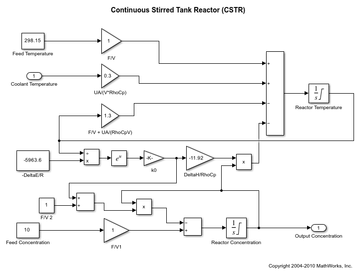
Continuous Stirred Tank Reactor
The nonlinearity in the CSTR plant yields different linearized dynamics at different output concentrations. The example uses the Gain-Scheduled PID Autotuner to tune a separate PID controller for each output concentration.
Overview
mdl = 'scdgainscheduledautocstrplant';Gain-Scheduled PID Autotuning Setup
Gain-Scheduled PID Autotuner
To implement gain-scheduling and autotuning the Gain-Scheduled PID Autotuner block from Simulink Control Design is used. This block allows for the implementation of gain-scheduling and provides a way to both tune the gains at multiple operating conditions and store the gains for use elsewhere in the model or system.
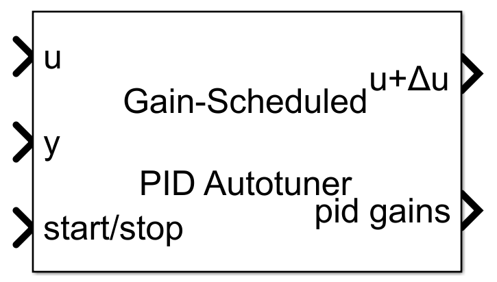
The autotuning workflow for this block is similar to the Closed-Loop PID Autotuner. The Gain-Scheduled PID Autotuner block allows you to tune one PID controller at a time. It injects perturbation signals at the plant input and measures the plant output during a closed-loop experiment. When the experiment stops, the block computes PID gains based on the plant frequency responses estimated at a small number of points near the desired bandwidth. The tuned PID gains are stored and the existing gain array, if available, is updated at the corresponding value of the scheduling variable (by default the scheduling variable is the same as the plant output). The Gain-Scheduled PID Autotuner block will also automatically determine the current PID gains based on the current value of the scheduling variable and output the corresponding gains for use in a PID Controller.
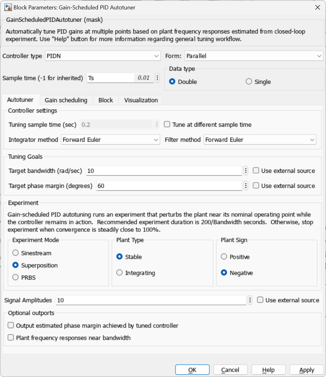
The Gain-Scheduled PID Autotuner is added to the model after the PID Controller and before the CSTR plant input for temperature. When not enabled (start/stop signal is 0), the autotuner will be a passthrough from the input u to the output u+deltaU and will output the PID gains corresponding to the value of the scheduling variable. To setup the Gain-Scheduled PID Autotuner for use in this example first the autotuning settings need to be set on the Autotuner tab:
Controller Type: PIDN to match the PID controller
Bandwidth: 10 rad/sec which is used in previous CSTR examples
Phase Margin: 60 degrees to balance overshoot and robustness
Signal Amplitudes: 10 to allow for sufficient perturbation amplitudes and keep away from down stream limits
Plant Sign: Negative since the CSTR plant is a negative plant
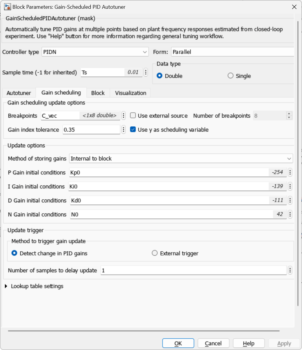
Next, the block is configured for gain scheduling on the Gain scheduling tab as follows:
Breakpoints: set to the parameter C_vec which will be defined later in this example
P Gain initial conditions: Kp0. This is the default Kp gain that will be defined later in this example
I Gain initial conditions: Ki0. This is the default Ki gain that will be defined later in this example
D Gain initial conditions: Kd0. This is the default Kd gain that will be defined later in this example
N Gain initial conditions: N0. This is the default N filter parameter that will be defined later in this example
The gains from the Gain-Scheduled PID Autotuner are output and fed back to the PID Controller block and are updated during simulation once they are tuned for a given operating point.
Visualization Plots
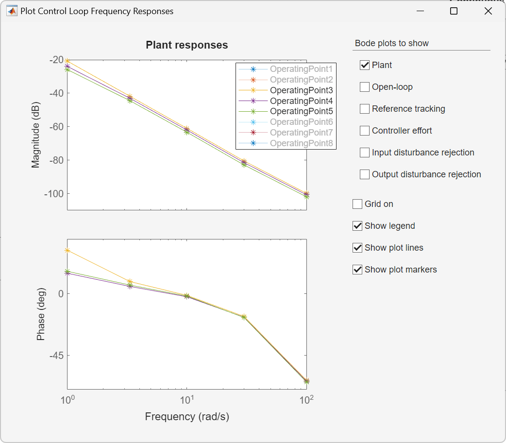
On the Visualization tab of the Gain-Scheduled PID Tuner two different plots can be used to visualize the estimated frequency responses or tuned gains at the various operating points. For the bode plot, up to six different frequency domain plots can be shown for the 5 frequency points estimated at each operating point:
Plant: open-loop plant response
Open-loop: response of the open-loop controller-plant system
Reference tracking: closed-loop system response to a step change in setpoint
Controller effort: closed-loop controller output response to a step change in setpoint
Input disturbance rejection: closed-loop system response to a load disturbance (step change at plant input)
Output disturbance rejection: closed-loop system response to a step disturbance at the plant output
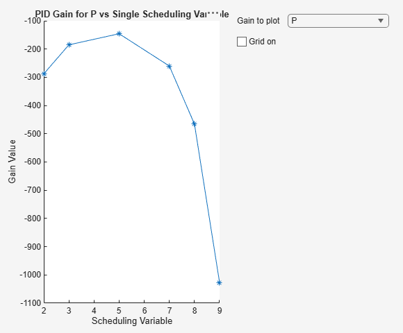
For the Gain surface plot, the 4 PIDN gains can be visualized plotted against the scheduling variable.
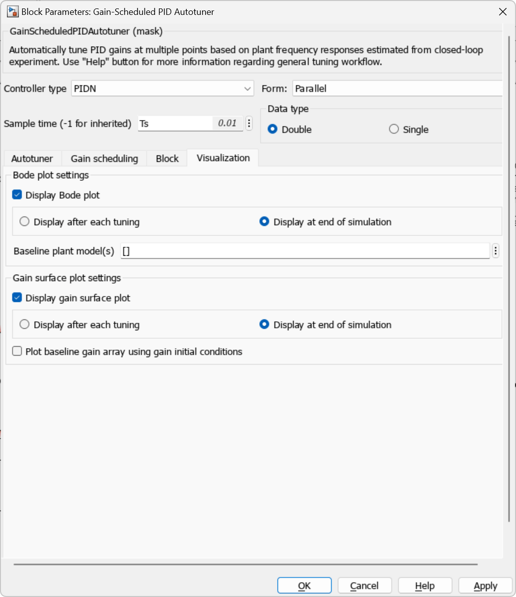
The plots can be refreshed while the simulation runs or at the end of the simulation. For this example both the bode plot for the frequency responses and the gain surface plot for the PIDN gains will be used and displayed only at the end of the simulation.
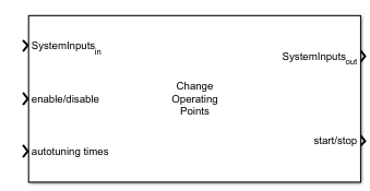
Change Operating Points
After the Gain-Scheduled PID Autotuner is setup the Change Operating Points block needs to be setup to provide the start/stop signal needed in the Gain-Scheduled PID Autotuner as well as change the target output concentration from 2 to 9.
The Change Operating Points is configured to move the system between all 8 output concentrations with the baseline PID controller, perform tuning then do the same initial transient. This is done to make a comparison for before and after tuning. The desired bandwidth, as mentioned above, is 10 rad/sec so the autotuning time is set to be 200/bandwidth or 20 seconds.
Initial Tuning
The Gain-Scheduled PID Autotuner requires a stabilizing controller in order to perform tuning at the different operating points. For the CSTR the following initial gains are used along with a sample time of 0.01 seconds. These gains were obtained by tuning the controller at a fixed operating point.
% Initial Controller Gains
Kp0 = -254;
Ki0 = -139;
Kd0 = -111;
N0 = 42;
Ts = 0.01;
For the initial tuning all 8 output concentration operating points are used.
% Reactor Concentration Operating Points
C_vec = [2 3 4 5 6 7 8 9];
The below vectors are used to create a vector for moving the CSTR plant from 2 to 9 incrementally, do the same but perform tuning, then repeat the initial transient.
% Get vectors to coordinate tuning
% Change OP Block
Cref_initial = [2 3 4 5 6 7 8 9];
Cref_tuning = C_vec;
Cref_final = [2 3 4 5 6 7 8 9];
Cref_vec = [Cref_initial Cref_tuning Cref_final];

% Build Time Vectors for Change OP Block
Time_initial = (0:1:length(Cref_initial))*10;
Time_tuning = (1:1:length(Cref_tuning))*30 + Time_initial(end);
Time_final = (1:1:length(Cref_final)-1)*10 + Time_tuning(end);
Time_vec = [Time_initial Time_tuning Time_final];

% Autotuning Parameters
EnableAutoTuning = Time_initial(end)+5*Ts;
DisableAutoTuning = Time_tuning(end);
AutotuningStartTimes = Time_tuning-25;

% Save Data Indices for plotting
idx_0 = Time_initial(end)/Ts;
idx1_gs = Time_tuning(end)/Ts;
idx2_gs = (Time_final(end)+10)/Ts;

% Open model after initializing
open_system(mdl)
When all the vectors are setup, the simulation can be run and the visualization plots will displayed when the simulation has ended.
% Run Simulation
baselineResults = sim(mdl);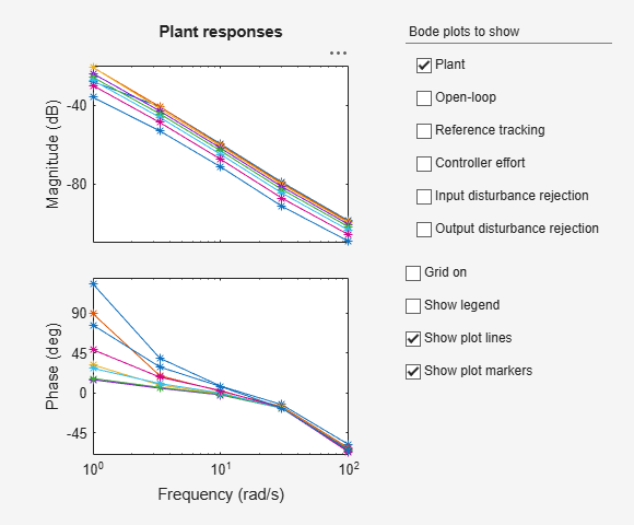
The first image shows the bode plot dialog used to display up to six different frequency responses as discussed previously. For this example, only the Plant responses will be used but the other 5 can be enabled/disabled as desired to view the different responses.
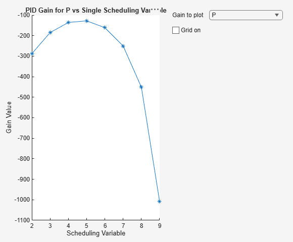
The second image shows gain surface plot used to display the PIDN gains vs the scheduling variable. By default, the P gain is plotted but the other three gains, IDN, can also be viewed through the drop down.
Inspecting the Plant Responses and Gain plots, the responses for operating points 3,4 and 5 (and their respective PIDN gains) have minimal differences. Showing just these three operating points on the Plant Responses plot it's clear to see that both the magnitude and phase responses of these operating points are similar.
In the initial tuning of the gain-scheduled PID controller 8 breakpoints were used. However, using the visualization plots, it's clear that operating points 3 and 5 can be eliminated (which correspond to output concentrations of 4 and 6, respectively) to reduce the number of operating points being tuned and, thus, reduce the length of time for the entire tuning process.
Reduced Operating Points
As discussed in the previous section the number of breakpoints can be reduced from 8 to 6 by removing the breakpoints at output concentrations of 4 and 6. Doing this the entire tuning process can be repeated.
% Reduce Reactor Concentration Operating Points
C_vec = [2 3 5 7 8 9];

% Get vectors to coordinate tuning
% Change OP Block
Cref_initial = [2 3 4 5 6 7 8 9];
Cref_tuning = C_vec;
Cref_final = [2 3 4 5 6 7 8 9];
Cref_vec = [Cref_initial Cref_tuning Cref_final];

% Build Time Vectors for Change OP Block
Time_initial = (0:1:length(Cref_initial))*10;
Time_tuning = (1:1:length(Cref_tuning))*30 + Time_initial(end);
Time_final = (1:1:length(Cref_final)-1)*10 + Time_tuning(end);
Time_vec = [Time_initial Time_tuning Time_final];

% Autotuning Parameters
EnableAutoTuning = Time_initial(end)+5*Ts;
DisableAutoTuning = Time_tuning(end);
AutotuningStartTimes = Time_tuning-25;

% Get final transient with GS gains
idx1_gs2 = Time_tuning(end)/Ts;
idx2_gs2 = (Time_final(end)+10)/Ts;
After recomputing the vectors above the simulation can be re-run and new visualization plots will be obtained.
% Run Simulation
reducedOPResults = sim(mdl);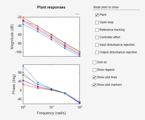
When the simulation is re-run the existing dialog will refresh with the updated frequency responses and updated gain plots. There is no need to closed the existing dialog.
With both simulation results available, as well as the initial transient performed with a single tuned PID controller, the 3 reposes can be compared to determine if it was appropriate to reduce the number of breakpoints from 8 to 6.
% Plot results
ExampleHelperPlotGSResults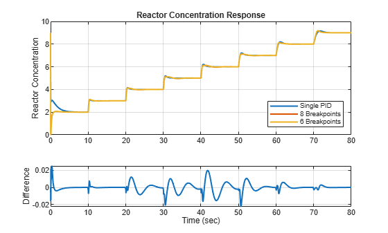
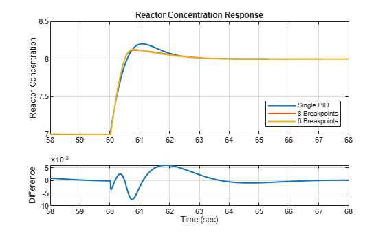
As shown in the above plots, the gain-scheduled PID controller has reduced overshoot and similar settling time compared to using just a single PID controller. When comparing the initial tuning results using 8 breakpoints with the results using 6 breakpoints the responses are similar with minimal differences. This result was achievable by using the visualization plots to analyze the data during and after the simulation and adjusting the number of breakpoints. There was no need to export any data to Matlab or inspect multiple signals.
Summary
The visualization plots for plant responses and gain surface on the Gain-Scheduled PID Autotuner provide a way to analyze the results of autotuning for a gain-scheduled PID controller during simulation. These plots allow for in model analysis of plant operating point responses and gains to assist in increasing or decreasing the number of points needed for a gain-scheduled PID controller.