Command Line Verification Tutorial
This example creates three test cases for an adjustable rate limiter and analyzes the resulting model coverage using the command-line API of the Model Coverage tool.
Simulink® Model for the Adjustable Rate Limiter
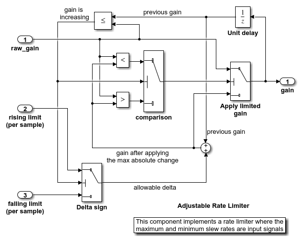
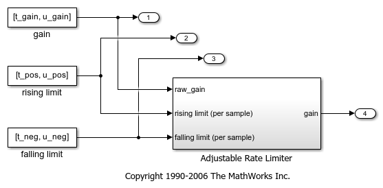
The Simulink® subsystem Adjustable Rate Limiter is a rate limiter in the model 'slvnvdemo_ratelim_harness'. It uses three switch blocks to control when the output should be limited and the type of limit to apply.
Inputs are produced with the From Workspace blocks 'gain', 'rising limit', and 'falling limit', which generate piecewise linear signals. The values of the inputs are specified with six variables defined in the MATLAB® workspace: t_gain, u_gain, t_pos, u_pos, t_neg, and u_neg.
Open the model and the Adjustable Rate Limiter subsystem.
modelName = 'slvnvdemo_ratelim_harness';
open_system(modelName);
open_system([modelName,'/Adjustable Rate Limiter']);
Creating the First Test Case
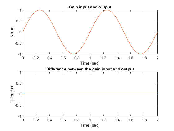
The first test case verifies that the output matches the input when the input values do not change rapidly. It uses a sine wave as the time varying signal and constants for rising and falling limits.
t_gain = (0:0.02:2.0)';
u_gain = sin(2*pi*t_gain);
Calculate the minimum and maximum change of the time varying input using the MATLAB diff function.
max_change = max(diff(u_gain))
min_change = min(diff(u_gain))
max_change =

    0.1253


min_change =

   -0.1253
Because the signal changes are much less than 1 and much greater than -1, set the rate limits to 1 and -1. The variables are all stored in the MAT file 'within_lim.mat', which is loaded before simulation.
t_pos = [0;2];
u_pos = [1;1];
t_neg = [0;2];
u_neg = [-1;-1];

save('within_lim.mat','t_gain','u_gain','t_pos','u_pos','t_neg','u_neg');
Additional Test Cases
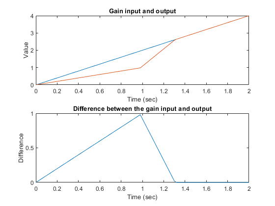
The second test case complements the first case with a rising gain that exceeds the rate limit. After a second it increases the rate limit so that the gain changes are below that limit.
t_gain = [0;2];
u_gain = [0;4];
t_pos = [0;1;1;2];
u_pos = [1;1;5;5]*0.02;
t_neg = [0;2];
u_neg = [0;0];

save('rising_gain.mat','t_gain','u_gain','t_pos','u_pos','t_neg','u_neg');
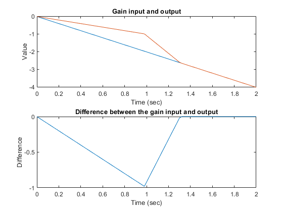
The third test case is a mirror image of the second, with the rising gain replaced by a falling gain.
t_gain = [0;2];
u_gain = [-0.02;-4.02];
t_pos = [0;2];
u_pos = [0;0];
t_neg = [0;1;1;2];
u_neg = [-1;-1;-5;-5]*0.02;

save('falling_gain.mat','t_gain','u_gain','t_pos','u_pos','t_neg','u_neg');
Defining Coverage Tests
The test cases are organized and executed using sim
In this example, a simulation input object is used to set the coverage configuration.
covSet = Simulink.SimulationInput(modelName);
covSet = setModelParameter(covSet,'CovEnable','on');
covSet = setModelParameter(covSet,'CovMetricStructuralLevel','Decision');
covSet = setModelParameter(covSet,'CovSaveSingleToWorkspaceVar','on');
covSet = setModelParameter(covSet,'CovScope','Subsystem');
covSet = setModelParameter(covSet,'CovPath','/Adjustable Rate Limiter');
covSet = setModelParameter(covSet,'StartTime','0.0');
covSet = setModelParameter(covSet,'StopTime','2.0');
Executing Coverage Tests
Load the data for the first test case, set the coverage variable name, and execute the model using sim.
load within_lim.mat
covSet = setModelParameter(covSet,'CovSaveName','dataObj1');
simOut1 = sim(covSet);
dataObj1
dataObj1 = ... cvdata
            version: (R2026a)
                 id: 1954
               type: TEST_DATA
               test: cvtest object
             rootID: 1956
           checksum: [1x1 struct]
          modelinfo: [1x1 struct]
          startTime: 19-Apr-2026 12:12:40
           stopTime: 19-Apr-2026 12:12:40
  intervalStartTime:
   intervalStopTime:
simulationStartTime: 0
 simulationStopTime: 2
             filter:
            simMode: Normal
Verify the first test case by checking that the output matches the input.
subplot(211)
plot(simOut1.tout,simOut1.yout(:,1),simOut1.tout,simOut1.yout(:,4))
xlabel('Time (sec)'), ylabel('Value'),
title('Gain input and output');
subplot(212)
plot(simOut1.tout,simOut1.yout(:,1)-simOut1.yout(:,4))
xlabel('Time (sec)'),ylabel('Difference'),
title('Difference between the gain input and output');
Execute and plot results for the second test case in the same way.
Notice that once the limited output has diverged from the input it can only recover at the maximum slew rate. This is why the plot has an unusual kink. Once the input and output match, the two change together.
load rising_gain.mat
covSet = setModelParameter(covSet,'CovSaveName','dataObj2');
simOut2 = sim(covSet);
dataObj2

subplot(211)
plot(simOut2.tout,simOut2.yout(:,1),simOut2.tout,simOut2.yout(:,4))
xlabel('Time (sec)'), ylabel('Value'),
title('Gain input and output');
subplot(212)
plot(simOut2.tout,simOut2.yout(:,1)-simOut2.yout(:,4))
xlabel('Time (sec)'), ylabel('Difference'),
title('Difference between the gain input and output');
dataObj2 = ... cvdata
            version: (R2026a)
                 id: 306
               type: TEST_DATA
               test: cvtest object
             rootID: 1956
           checksum: [1x1 struct]
          modelinfo: [1x1 struct]
          startTime: 19-Apr-2026 12:12:42
           stopTime: 19-Apr-2026 12:12:43
  intervalStartTime:
   intervalStopTime:
simulationStartTime: 0
 simulationStopTime: 2
             filter:
            simMode: Normal
Execute and plot results for the third test case.
load falling_gain.mat
covSet = setModelParameter(covSet,'CovSaveName','dataObj3');
simOut3 = sim(covSet);
dataObj3

subplot(211)
plot(simOut3.tout,simOut3.yout(:,1),simOut3.tout,simOut3.yout(:,4))
xlabel('Time (sec)'), ylabel('Value'),
title('Gain input and output');
subplot(212)
plot(simOut3.tout,simOut3.yout(:,1)-simOut3.yout(:,4))
xlabel('Time (sec)'), ylabel('Difference'),
title('Difference between the gain input and output');
dataObj3 = ... cvdata
            version: (R2026a)
                 id: 428
               type: TEST_DATA
               test: cvtest object
             rootID: 1956
           checksum: [1x1 struct]
          modelinfo: [1x1 struct]
          startTime: 19-Apr-2026 12:12:44
           stopTime: 19-Apr-2026 12:12:44
  intervalStartTime:
   intervalStopTime:
simulationStartTime: 0
 simulationStopTime: 2
             filter:
            simMode: Normal
Generating a Coverage Report
Assuming that all the tests have passed, produce a combined report from all test cases to verify the achievement of 100% coverage. Coverage percentages for each test are displayed under the heading "Model Hierarchy." Although none of the tests individually achieved 100% coverage, in aggregate, they achieve complete coverage.
cvhtml('combined_ratelim',dataObj1,dataObj2,dataObj3);
Saving Coverage Data
Save the collected coverage data in the file "ratelim_testdata.cvt" by using cvsave.
cvsave('ratelim_testdata',dataObj1,dataObj2,dataObj3);
Close the model and exit the coverage environment
close_system('slvnvdemo_ratelim_harness',0);
clear dataObj*
Loading Coverage Data
Restore saved coverage tests from the file "ratelim_testdata.cvt" after opening the model by using cvload. The data and tests are retrieved in a cell array.
open_system('slvnvdemo_ratelim_harness');
[SavedTests,SavedData] = cvload('ratelim_testdata')
SavedTests =

  1×3 cell array

    {1×1 cvtest}    {1×1 cvtest}    {1×1 cvtest}


SavedData =

  1×3 cell array

    {1×1 cvdata}    {1×1 cvdata}    {1×1 cvdata}
Manipulating Coverage Data Objects
Manipulate cvdata objects using the overloaded operators: +, -, and *. The * operator is used to find the intersection of two coverage data objects, which results in another cvdata object. For example, the following command produces an HTML report of the common coverage from all three tests.
common = SavedData{1} * SavedData{2} * SavedData{3}
cvhtml('intersection',common);
common = ... cvdata
            version: (R2026a)
                 id: 0
               type: DERIVED_DATA
               test: []
             rootID: 553
           checksum: [1x1 struct]
          modelinfo: [1x1 struct]
          startTime: 19-Apr-2026 12:12:40
           stopTime: 19-Apr-2026 12:12:44
  intervalStartTime:
   intervalStopTime:
             filter:
            simMode: Normal
Extracting Information from Coverage Data Objects
Retrieve decision coverage information from a block path or block handle by using decisioninfo. The output is a vector with the achieved and total outcomes for a single model object, respectively.
cov = decisioninfo(SavedData{1} + SavedData{2} + SavedData{3}, ...
                   'slvnvdemo_ratelim_harness/Adjustable Rate Limiter')
cov =

     6     6
Use the retrieved coverage information to access the percentage coverage.
percentCov = 100 * (cov(1)/cov(2))
percentCov = 100
When two output arguments are used, decisioninfo returns a structure that captures the decisions and outcomes within the Simulink block or Stateflow® object.
[blockCov,desc] = decisioninfo(common, ...
         'slvnvdemo_ratelim_harness/Adjustable Rate Limiter/Delta sign')
descDecision = desc.decision
outcome1 = desc.decision.outcome(1)
outcome2 = desc.decision.outcome(2)
blockCov =

     0     2


desc =

  struct with fields:

           isFiltered: 0
    justifiedCoverage: 0
          isJustified: 0
      filterRationale: ''
             decision: [1×1 struct]


descDecision =

  struct with fields:

               text: 'Switch trigger'
    filterRationale: ''
         isFiltered: 0
        isJustified: 0
            outcome: [1×2 struct]


outcome1 =

  struct with fields:

               text: 'false (out = in3)'
     executionCount: 0
         executedIn: []
         isFiltered: 0
        isJustified: 0
    filterRationale: ''


outcome2 =

  struct with fields:

               text: 'true (out = in1)'
     executionCount: 0
         executedIn: []
         isFiltered: 0
        isJustified: 0
    filterRationale: ''