cophenet

Cophenetic correlation coefficient

Syntax

c = cophenet(Z,Y)

[c,D] = cophenet(Z,Y)

Description

c = cophenet(Z,Y) returns the cophenetic correlation coefficient for the hierarchical cluster tree represented by Z, where Y contains the distances (or dissimilarities) used to create Z.

[c,D] = cophenet(Z,Y) additionally returns the cophenetic correlation distances D in the same lower triangular distance vector format as Y.

Examples

Cophenetic Correlation Coefficient

Load the examgrades data set.

load examgrades

Create a hierarchical cluster tree using the linkage function. Specify the average method and the Minkowski distance metric with an exponent of 3.

Z = linkage(grades,"average",{"minkowski",3});

Compute the distances between pairs of observations using the pdist function.

Y = pdist(grades);

Compute the cophenetic correlation coefficient.

c = cophenet(Z,Y)

c = 
0.6308

The moderately high correlation coefficient suggests that the hierarchical clustering tree provides a reasonably good representation of the distances between observations.

Cophenetic Correlation Coefficient and Distances

Create a sample data set consisting of randomly generated data from three standard uniform distributions.

rng(0,"twister");  % For reproducibility
X = [gallery("uniformdata",[10 3],12); ...
    gallery("uniformdata",[10 3],13)+1.2; ...
    gallery("uniformdata",[10 3],14)+2.5];
c = [ones(10,1);2*(ones(10,1));3*(ones(10,1))]; % Actual classes

Create a scatter plot of the data.

scatter3(X(:,1),X(:,2),X(:,3),100,c,"filled")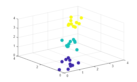

Create a hierarchical cluster tree using the linkage function. Specify the weighted method and the standardized Euclidean distance metric.

Z = linkage(X,"weighted","seuclidean");

Compute the distances between pairs of observations using the pdist function, and display a dendrogram plot.

Y = pdist(X);
dendrogram(Z)

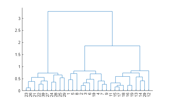
Return the cophenetic correlation coefficient and cophenetic distances.

[c,D] = cophenet(Z,Y)

c = 
0.8179

D = 1×435

    0.8203    0.8203    0.8203    0.4604    0.8203    0.8203    0.7150    0.8203    0.8203    1.8599    1.8599    1.8599    1.8599    1.8599    1.8599    1.8599    1.8599    1.8599    1.8599    3.2866    3.2866    3.2866    3.2866    3.2866    3.2866    3.2866    3.2866    3.2866    3.2866    0.2213    0.7024    0.8203    0.3286    0.7024    0.8203    0.7024    0.4772    1.8599    1.8599    1.8599    1.8599    1.8599    1.8599    1.8599    1.8599    1.8599    1.8599    3.2866    3.2866    3.2866

The high correlation coefficient suggests that the dendrogram provides a good representation of the pairwise distances Y.

Create a second hierarchical cluster tree using the complete method, which computes the largest distance between objects in each cluster.

ZZ = linkage(X,"complete","seuclidean");

Compute the distances between pairs of observations. Return the cophenetic correlation coefficient and the cophenetic distances.

YY = pdist(X);
[cc,DD] = cophenet(ZZ,YY)

cc = 
0.8202

DD = 1×435

    1.2044    1.2044    1.2044    0.4604    1.2044    1.2044    1.2044    1.2044    1.2044    2.9605    2.9605    2.9605    2.9605    2.9605    2.9605    2.9605    2.9605    2.9605    2.9605    5.0417    5.0417    5.0417    5.0417    5.0417    5.0417    5.0417    5.0417    5.0417    5.0417    0.2213    0.8986    1.2044    0.3696    0.8986    0.8595    0.8986    0.5287    2.9605    2.9605    2.9605    2.9605    2.9605    2.9605    2.9605    2.9605    2.9605    2.9605    5.0417    5.0417    5.0417

Create a scatter plot of pairwise distance versus cophenetic distance for the two cluster trees.

scatter(D,Y)
hold on
scatter(DD,YY,"x")
plot([0,max(Y)],[0,max(Y)],"b:",LineWidth=2); % Plot the 1:1 line
xlabel("Cophenetic Distance");
ylabel("Pairwise Distance")
legend("Weighted","Complete","1:1 line",Location="northwest")
hold off

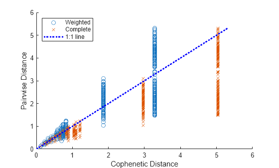
The cluster trees have similar cophenetic correlation coefficients, but the cophenetic distances of the tree created with the complete method are systematically larger than their corresponding pairwise distances.

Input Arguments

Z — Hierarchical cluster tree

numeric matrix

Hierarchical cluster tree, specified as a numeric matrix returned by the linkage function. Z has size (m – 1)-by-3, where m is the number of observations used to create the cluster tree. The third column of Z contains linkage distances. For more information, see Agglomerative hierarchical cluster tree.

Data Types: single | double

Y — Distances (or dissimilarities) used to create Z

numeric row vector

Distances (or dissimilarities) used to create Z, specified as a numeric row vector returned by the pdist function. Y has length m*(m – 1)/2, where m is the number of observations used to create the cluster tree.

Data Types: single | double

Output Arguments

c — Cophenetic correlation coefficient

numeric scalar

Cophenetic correlation coefficient, returned as a numeric scalar. The cophenetic correlation for a cluster tree is the linear correlation coefficient between the cophenetic distances obtained from the tree, and the original distances (or dissimilarities) used to create the tree. So, the cophenetic correlation coefficient is a measure of how faithfully the tree represents the dissimilarities among observations. A cophenetic correlation coefficient with a magnitude close to 1 indicates a high-quality solution. You can use this measure to compare alternative cluster solutions obtained using different algorithms.

The cophenetic correlation between Z(:,3) and Y is defined as

$$c=\frac{{\sum }_{i<j}(Y_{ij}-y)(Z_{ij}-z)}{\sqrt{{\sum }_{i<j}{(Y_{ij}-y)}^2{\sum }_{i<j}{(Z_{ij}-z)}^2}}$$

where:

• Y_ij is the distance between objects i and j in Y.

• Z_ij is the cophenetic distance between objects i and j, from Z(:,3).

• y and z are the averages of Y and Z(:,3), respectively.

D — Cophenetic distances

numeric row vector

Cophenetic distances, returned as a numeric row vector with the same length as Y. The cophenetic distance between two observations is represented in a dendrogram by the height of the link at which the two observations are first joined. This height is the distance between the two subclusters that are merged by the link.

Version History

Introduced before R2006a