Residuals
Purpose
Residuals are useful for detecting outlying y values and checking the linear regression assumptions with respect to the error term in the regression model. High-leverage observations have smaller residuals because they often shift the regression line or surface closer to them. You can also use residuals to detect some forms of heteroscedasticity and autocorrelation.
Definition
The Residuals matrix is an n-by-4 table containing four types of residuals, with one row for each observation.
Raw Residuals
Observed minus fitted values, that is,
Pearson Residuals
Raw residuals divided by the root mean squared error, that is,
where ri is the raw residual and MSE is the mean squared error.
Standardized Residuals
Standardized residuals are raw residuals divided by their estimated standard deviation. The standardized residual for observation i is
where MSE is the mean squared error and hii is the leverage value for observation i.
Studentized Residuals
Studentized residuals are the raw residuals divided by an independent estimate of the residual standard deviation. The residual for observation i is divided by an estimate of the error standard deviation based on all observations except for observation i.
where MSE(i) is the mean squared error of the regression fit calculated by removing observation i, and hii is the leverage value for observation i. The studentized residual sri has a t-distribution with n – p – 1 degrees of freedom.
How To
After obtaining a fitted model, say, mdl, using fitlm or stepwiselm, you can:
Find the
Residualstable undermdlobject.Obtain any of these columns as a vector by indexing into the property using dot notation, for example,
mdl.Residuals.Raw
Plot any of the residuals for the values fitted by your model using
For details, see theplotResiduals(mdl)
plotResidualsmethod of theLinearModelclass.
Assess Model Assumptions Using Residuals
This example shows how to assess the model assumptions by examining the residuals of a fitted linear regression model.
Load the sample data and store the independent and response variables in a table.
 load imports-85
 tbl = table(X(:,7),X(:,8),X(:,9),X(:,15),'VariableNames',...
{'curb_weight','engine_size','bore','price'});
Fit a linear regression model.
mdl = fitlm(tbl)
mdl =
Linear regression model:
    price ~ 1 + curb_weight + engine_size + bore

Estimated Coefficients:
                    Estimate        SE         tStat       pValue
                   __________    _________    _______    __________

    (Intercept)        64.095        3.703     17.309    2.0481e-41
    curb_weight    -0.0086681    0.0011025    -7.8623      2.42e-13
    engine_size     -0.015806     0.013255    -1.1925       0.23452
    bore              -2.6998       1.3489    -2.0015      0.046711


Number of observations: 201, Error degrees of freedom: 197
Root Mean Squared Error: 3.95
R-squared: 0.674,  Adjusted R-Squared: 0.669
F-statistic vs. constant model: 136, p-value = 1.14e-47
Plot the histogram of raw residuals.
plotResiduals(mdl)
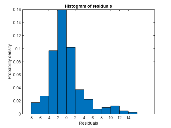
The histogram shows that the residuals are slightly right skewed.
Plot the box plot of all four types of residuals.
 Res = table2array(mdl.Residuals);
 boxplot(Res)
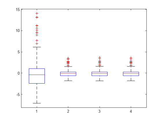
You can see the right-skewed structure of the residuals in the box plot as well.
Plot the normal probability plot of the raw residuals.
plotResiduals(mdl,'probability')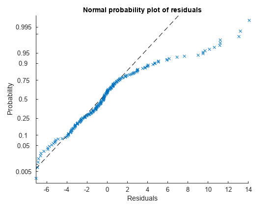
This normal probability plot also shows the deviation from normality and the skewness on the right tail of the distribution of residuals.
Plot the residuals versus lagged residuals.
plotResiduals(mdl,'lagged')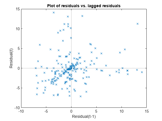
This graph shows a trend, which indicates a possible correlation among the residuals. You can further check this using dwtest(mdl). Serial correlation among residuals usually means that the model can be improved.
Plot the symmetry plot of residuals.
plotResiduals(mdl,'symmetry')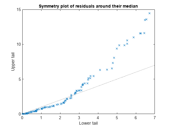
This plot also suggests that the residuals are not distributed equally around their median, as would be expected for normal distribution.
Plot the residuals versus the fitted values.
plotResiduals(mdl,'fitted')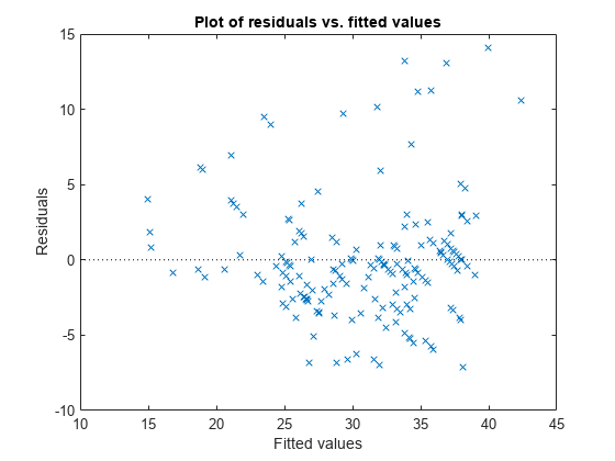
The increase in the variance as the fitted values increase suggests possible heteroscedasticity.
References
[1] Atkinson, A. T. Plots, Transformations, and Regression. An Introduction to Graphical Methods of Diagnostic Regression Analysis. New York: Oxford Statistical Science Series, Oxford University Press, 1987.
[2] Neter, J., M. H. Kutner, C. J. Nachtsheim, and W. Wasserman. Applied Linear Statistical Models. IRWIN, The McGraw-Hill Companies, Inc., 1996.
[3] Belsley, D. A., E. Kuh, and R. E. Welsch. Regression Diagnostics, Identifying Influential Data and Sources of Collinearity. Wiley Series in Probability and Mathematical Statistics, John Wiley and Sons, Inc., 1980.
See Also
LinearModel | fitlm | stepwiselm | plotDiagnostics | plotResiduals | dwtest