Tune Classification Model Using Experiment Manager

This example shows how to use Experiment Manager to optimize a machine learning classifier. The goal is to create a classifier for the CreditRating_Historical data set that has minimal cross-validation loss. Begin by using the Classification Learner app to train all available classification models on the training data. Then, improve the best model by exporting it to Experiment Manager.

In Experiment Manager, use the default settings to minimize the cross-validation loss (that is, maximize the cross-validation accuracy). Investigate options that help improve the loss, and perform more detailed experiments. For example, fix some hyperparameters at their best values, add useful hyperparameters to the model tuning process, adjust hyperparameter search ranges, adjust the training data, and customize the visualizations. The final result is a classifier with better test set accuracy.

For more information on when to export models from Classification Learner to Experiment Manager, see Export Model from Classification Learner to Experiment Manager.

Load and Partition Data

In the MATLAB^® Command Window, read the sample file CreditRating_Historical.dat into a table. The predictor data contains financial ratios and industry sector information for a list of corporate customers. The response variable contains credit ratings assigned by a rating agency.
```
creditrating = readtable("CreditRating_Historical.dat");
```
The goal is to create a classification model that predicts a customer's rating, based on the customer's information.
Because each value in the ID variable is a unique customer ID, that is, length(unique(creditrating.ID)) is equal to the number of observations in creditrating, the ID variable is a poor predictor. Remove the ID variable from the table, and convert the Industry variable to a categorical variable.
```
creditrating = removevars(creditrating,"ID");
creditrating.Industry = categorical(creditrating.Industry);
```
Convert the response variable Rating to a categorical variable and specify the order of the categories.
```
creditrating.Rating = categorical(creditrating.Rating, ...
    ["AAA","AA","A","BBB","BB","B","CCC"]);
```
Partition the data into two sets. Use approximately 80% of the observations for model training in Classification Learner, and reserve 20% of the observations for a final test set. Use cvpartition to partition the data.
```
rng("default") % For reproducibility
c = cvpartition(creditrating.Rating,"Holdout",0.2);
trainingIndices = training(c);
testIndices = test(c);
creditTrain = creditrating(trainingIndices,:);
creditTest = creditrating(testIndices,:);
```

Train Models in Classification Learner

If you have Parallel Computing Toolbox™, the Classification Learner app can train models in parallel. Training models in parallel is typically faster than training models in series. If you do not have Parallel Computing Toolbox, skip to the next step.
Before opening the app, start a parallel pool of process workers by using the parpool function.
```
parpool("Processes")
```
By starting a parallel pool of process workers rather than thread workers, you ensure that Experiment Manager can use the same parallel pool later.

Note
Parallel computations with a thread pool are not supported in Experiment Manager.
Open Classification Learner. Click the Apps tab, and then click the arrow at the right of the Apps section to open the apps gallery. In the Machine Learning and Deep Learning group, click Classification Learner.
On the Learn tab, in the File section, click New Session and select From Workspace.
In the New Session from Workspace dialog box, select the creditTrain table from the Data Set Variable list. The app selects the response and predictor variables. The default response variable is Rating. The default validation option is 5-fold cross-validation, to protect against overfitting.
In the Test section, click the check box to set aside a test data set. Specify 15 percent of the imported data as a test set.
To accept the options and continue, click Start Session.
To obtain the best classifier, train all preset models. On the Learn tab, in the Models section, click the arrow to open the gallery. In the Get Started group, click All. In the Train section, click Train All and select Train All. The app trains one of each preset model type, along with the default fine tree model, and displays the models in the Models pane.
To find the best result, sort the trained models based on the validation accuracy. In the Models pane, open the Sort by list and select Accuracy (Validation).
Note
Validation introduces some randomness into the results. Your model validation results can vary from the results shown in this example.

Assess Best Model Performance

For the model with the greatest validation accuracy, inspect the accuracy of the predictions in each class. Select the efficient linear SVM model in the Models pane. On the Learn tab, in the Plots and Results section, click the arrow to open the gallery, and then click Confusion Matrix (Validation) in the Validation Results group. View the matrix of true class and predicted class results. Blue values indicate correct classifications, and red values indicate incorrect classifications.
Overall, the model performs well. In particular, most of the misclassifications have a predicted value that is only one category away from the true value.
See how the classifier performed per class. Under Plot, select the True Positive Rates (TPR), False Negative Rates (FNR) option. The TPR is the proportion of correctly classified observations per true class. The FNR is the proportion of incorrectly classified observations per true class.
The model correctly classifies almost 94% of the observations with a true rating of AAA, but has difficulty classifying observations with a true rating of B.
Check the test set performance of the model. On the Test tab, in the Test section, click Test Selected. The app computes the test set performance of the model trained on the full data set, including training and validation data.
Compare the validation and test accuracy for the model. On the model Summary tab, compare the Accuracy (Validation) value under Training Results to the Accuracy (Test) value under Test Results. In this example, the two values are similar.

Export Model to Experiment Manager

To try to improve the classification accuracy of the model, export it to Experiment Manager. On the Learn tab, in the Export section, click Export Model and select Create Experiment. The Create Experiment dialog box opens.
Because the Rating response variable has multiple classes, the efficient linear SVM model is a multiclass ECOC model, trained using the fitcecoc function (with linear binary learners).
In the Create Experiment dialog box, click Create Experiment. The app opens Experiment Manager and a new dialog box.
In the dialog box, choose a new or existing project for your experiment. For this example, create a new project, and specify TrainEfficientModelProject as the filename in the Specify Project Folder Name dialog box.

Run Experiment with Default Hyperparameters

Run the experiment either sequentially or in parallel.
Note
- If you have Parallel Computing Toolbox, save time by running the experiment in parallel. On the Experiment Manager tab, in the Execution section, select Simultaneous from the Mode list.
- Otherwise, use the default Mode option of Sequential.
On the Experiment Manager tab, in the Run section, click Run.
Experiment Manager opens a new tab that displays the results of the experiment. At each trial, the app trains a model with a different combination of hyperparameter values, as specified in the Hyperparameters table in the Experiment1 tab.
After the app runs the experiment, check the results. In the table of results, click the arrow for the ValidationAccuracy column and select Sort in Descending Order.
Notice that the models with the greatest validation accuracy all have the same Coding value, onevsone.
Check the confusion matrix for the model with the greatest accuracy. On the Experiment Manager tab, in the Review Results section, click Confusion Matrix (Validation). In the Visualizations pane, the app displays the confusion matrix for the model.
For this model, all misclassifications have a predicted value that is only one category away from the true value.

Adjust Hyperparameters and Hyperparameter Values

The one-versus-one coding design seems best for this data set. To try to obtain a better classifier, fix the Coding hyperparameter value as onevsone and then rerun the experiment. Click the Experiment1 tab. In the Hyperparameters table, select the row for the Coding hyperparameter. Then click Delete.
To specify the coding design value, open the training function file. In the Training Function section, click Edit. The app opens the Experiment1_training1.mlx file.

In the file, search for the lines of code that use the fitcecoc function. This function is used to create multiclass linear classifiers. Specify the coding design value as a name-value argument. In this case, adjust the two calls to fitcecoc by adding 'Coding','onevsone' as follows.

classificationLinear = fitcecoc(predictors, response, ...
    'Learners', template, ecocParamsNameValuePairs{:}, ...
    'ClassNames', classNames, 'Coding', 'onevsone');

classificationLinear = fitcecoc(trainingPredictors, ...
    trainingResponse, 'Learners', template, ...
    ecocParamsNameValuePairs{:}, 'ClassNames', classNames, ...
    'Coding', 'onevsone');

Save the code changes, and close the file.

On the Experiment Manager tab, in the Run section, click Run.
To further vary the models evaluated during the experiment, add the regularization hyperparameter to the model tuning process. On the Experiment1 tab, in the Hyperparameters section, click Add. Edit the row entries so that the hyperparameter name is Regularization, the range is ["lasso","ridge"], and the type is categorical.
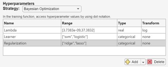
For more information on the hyperparameters you can tune for your model, see Export Model from Classification Learner to Experiment Manager.
On the Experiment Manager tab, in the Run section, click Run.
Adjust the range of values for the regularization term (lambda). On the Experiment1 tab, in the Hyperparameters table, change the Lambda range so that the upper bound is 3.7383e-02.
On the Experiment Manager tab, in the Run section, click Run.

Specify Training Data

Before running the experiment again, specify to use all the observations in creditTrain. Because you reserved some observations for testing when you imported the training data into Classification Learner, all experiments so far have used only 85% of the observations in the creditTrain data set.
Save the creditTrain data set as the file fullTrainingData.mat in the TrainEfficientModelProject folder, which contains the experiment files. To do so, right-click the creditTrain variable name in the MATLAB workspace, and click Save As. In the dialog box, specify the filename and location, and then click Save.
On the Experiment1 tab, in the Training Function section, click Edit.
In the Experiment1_training1.mlx file, search for the load command. Specify to use the full creditTrain data set for model training by adjusting the code as follows.
```
% Load training data
fileData = load("fullTrainingData.mat");
trainingData = fileData.creditTrain;
```
On the Experiment1 tab, in the Description section, change the number of observations to 3146, which is the number of rows in the creditTrain table.
On the Experiment Manager tab, in the Run section, click Run.
Instead of using all predictors, you can use a subset of the predictors to train and tune your model. In this case, omit the Industry variable from the model training process.
On the Experiment1 tab, in the Training Function section, click Edit.
In the Experiment1_training1.mlx file, search for the lines of code that specify the variables predictorNames and isCategoricalPredictor. Remove references to the Industry variable by adjusting the code as follows.
```
predictorNames = {'WC_TA', 'RE_TA', 'EBIT_TA', 'MVE_BVTD', 'S_TA'};
```
```
isCategoricalPredictor = [false, false, false, false, false];
```
On the Experiment1 tab, in the Description section, change the number of predictors to 5.
On the Experiment Manager tab, in the Run section, click Run.

Customize Confusion Matrix

You can customize the visualization returned by Experiment Manager at each trial. In this case, customize the validation confusion matrix so that it displays the true positive rates and false negative rates. On the Experiment1 tab, in the Training Function section, click Edit.
In the Experiment1_training1.mlx file, search for the confusionchart function. This function creates the validation confusion matrix for each trained model. Specify to display the number of correctly and incorrectly classified observations for each true class as percentages of the number of observations of the corresponding true class. Adjust the code as follows.
```
cm = confusionchart(response, validationPredictions, ...
    'RowSummary', 'row-normalized');
```
On the Experiment Manager tab, in the Run section, click Run.
In the table of results, click the arrow for the ValidationAccuracy column and select Sort in Descending Order.
Check the confusion matrix for the model with the greatest accuracy. On the Experiment Manager tab, in the Review Results section, click Confusion Matrix (Validation). In the Visualizations pane, the app displays the confusion matrix for the model.
Like the best-performing model trained in Classification Learner, this model has difficulty classifying observations with a true rating of B. However, this model is better at classifying observations with a true rating of CCC.

Export and Use Final Model

You can export a model trained in Experiment Manager to the MATLAB workspace. Select the best-performing model from the most recently run experiment. On the Experiment Manager tab, in the Export section, click Export and select Training Output.
In the Export dialog box, change the workspace variable name to finalLinearModel and click OK.
The new variable appears in your workspace.
Use the exported finalLinearModel structure to make predictions using new data. You can use the structure in the same way that you use any trained model exported from the Classification Learner app. For more information, see Make Predictions for New Data Using Exported Model.
In this case, predict labels for the test data in creditTest.
```
testLabels = finalLinearModel.predictFcn(creditTest);
```
Create a confusion matrix using the true test data response and the predicted labels.
```
cm = confusionchart(creditTest.Rating,testLabels, ...
    "RowSummary","row-normalized");
```
Compute the model test set accuracy using the values in the confusion matrix.
```
testAccuracy = sum(diag(cm.NormalizedValues))/ ...
    sum(cm.NormalizedValues,"all")
```
```
0.8015
```
The test set accuracy for this tuned model (80.2%) is greater than the test set accuracy for the efficient linear SVM classifier in Classification Learner (76.4%). However, keep in mind that the tuned model uses observations in creditTest as test data and the Classification Learner model uses a subset of the observations in creditTrain as test data.